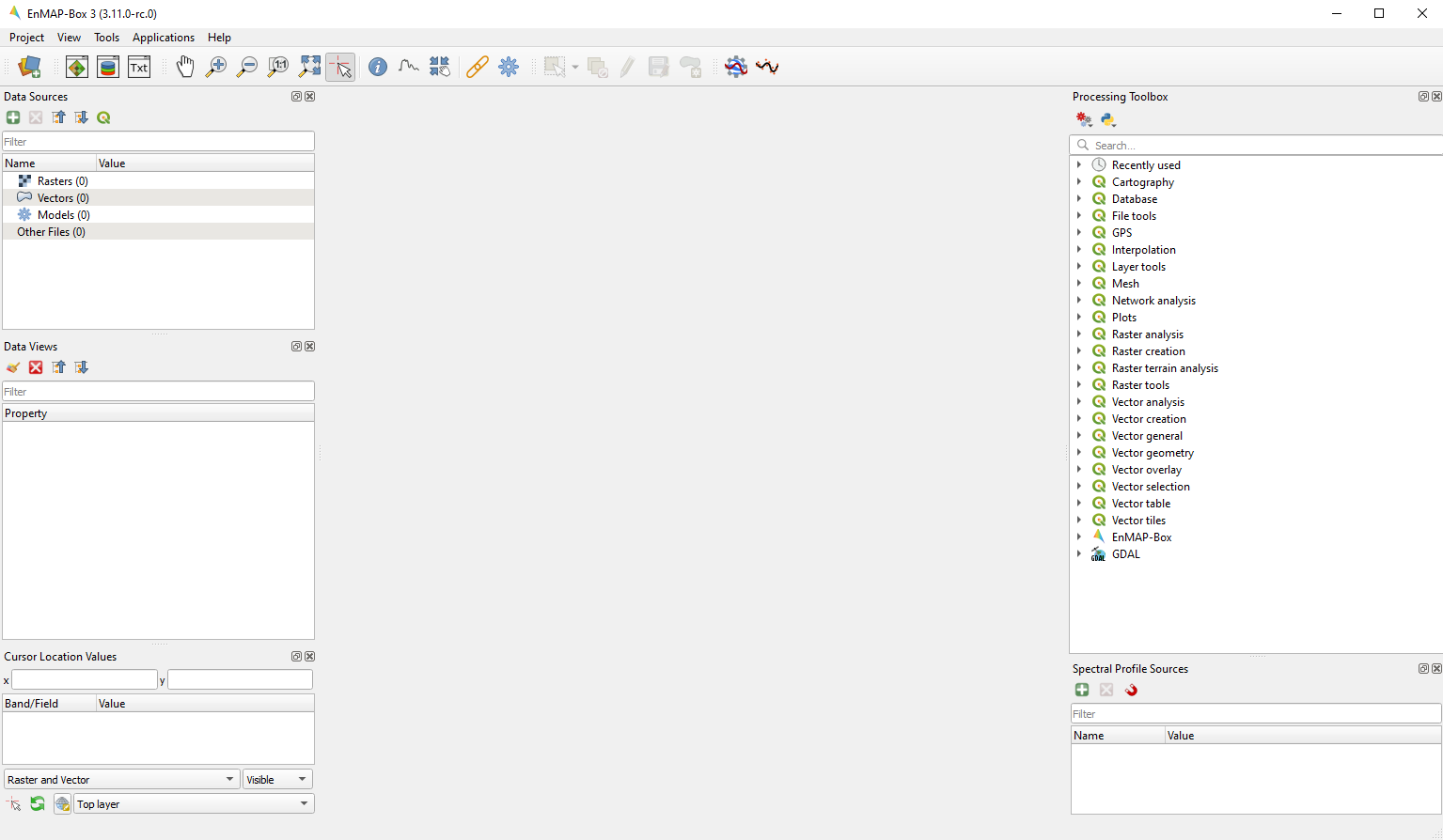
The Data Sources panel lists the data in your current project, comparable to the Layers panel in QGIS. The following data types and their
corresponding metadata are available:
Raster Data
File size: Metadata on resolution and extent of the raster
CRS: Shows Coordinate Reference System (CRS) information
Bands: Information on overall number of bands as well as band-wise metadata such as name, class or wavelength (if available)
Note
Depending on the type, raster layers will be listed with different icons:
for default raster layers (continuous value range)
for mask raster layers
for classification raster layers
Also see section on data types for further information.
Vector Data
File size: Shows the file size and extent of the vector layer
CRS: Shows Coordinate Reference System (CRS) information
Features: Information on number of features and geometry types
Fields: Attribute information, number of fields as well as field names and corresponding datatype
Spectral Libraries
File size: Size of the file on hard disk
Profiles: Shows the number of spectra in the library
Models
Buttons of the Data Sources panel:
Button
Description
This button lets you add data from different sources, e.g. raster and vector. Same function as .
Remove layers from the Data Sources panel. First select one or more and then click the remove button.
Collapses the whole menu tree, so that only layer type groups are shown.
Expands menu tree to show all branches.
Synchronizes Data Sources with QGIS.
Tip
If you want to remove all layers at once, right-click in the Data Sources panel and and select Remove all DataSources
The EnMAP-Box also supports Tile-/Web Map Services (e.g. Google Satellite or OpenStreetMap) as a raster layer. Just add them to
your QGIS project as you normally would, and then click the Synchronize Data Sources with QGIS
button. Now they should appear in the data source panel and can be added to a Map View.
The Data Views panel organizes the different windows and their content.
You may change the name of a Window by double-clicking onto the name in the list.
Buttons of the Data Views panel:
Button
Description
Open the Raster Layer Styling panel
Remove layers from the Data Views panel. First select one or more and then click the remove button.
Collapses the whole menu tree, so that only layer type groups are shown.
Expands menu tree to show all branches.
Organization of the Data Views panel:
Example of how different window types and their contents are organized in the Data Views panel. In this case there
are two Map Views and one Spectral Library View in the project.
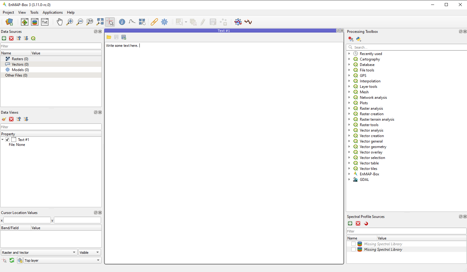
This menu manages the connection between raster sources and spectral library windows.
When collecting profiles, the Identify tool selects profiles from the top-most raster layer by default. The Profile Source panel allows to change this behaviour
and to control:
the profile source, i.e., the raster layer to collect profiles from,
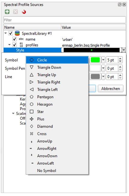
the style how they appear in the profile plot as profile candidate,
the sampling method, for example to aggregate multiple pixel into a single profile first,
the scaling of profile value.
Overview of the Spectral Profile Sources Window with two labeled spectra and main functionalities
Buttons of the Profile Sources
Button
Description
add a new profile source entry
remove selected entries
Profiles
Define the input data from where to take the spectral information from.
Style
Change style of displayed spectra, i.e. symbol and color
Source
Specify a source raster dataset
Double-clicking in the cell will open up a dropdown menu where you can select from all loaded raster datasets.
Sampling
Select Single Profile or Kernel by double-clicking into the cell.
Scaling
Choose how spectra are sampled.
Define the scaling factors by setting the Offset and Scale value.
Option
Description
SingleProfile
Extracts the spectral signature of the pixel at the selected location
Sample3x3
Extracts spectral signatures of the pixel at the selected location and its adjacent pixels in a 3x3 neighborhood.
Sample5x5
Extracts spectral signatures of the pixel at the selected location and its adjacent pixels in a 5x5 neighborhood.
Sample3x3Mean
Extracts the mean spectral signature of the pixel at the selected location and its adjacent pixels in a 3x3 neighborhood.
Sample5x5Mean
Extracts the mean spectral signature of the pixel at the selected location and its adjacent pixels in a 5x5 neighborhood.
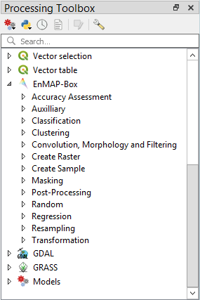
The processing toolbox is basically the same panel as in QGIS. Here you can find all EnMAP-Box processing algorithms
listed under EnMAP-Box. In case it is closed/not visible you can open it by clicking the
button in the menubar or View ‣ Panels ‣ QGIS Processing Toolbox.
This tools lets you inspect the values of a layer or multiple layers at the location where you click in the map view. To select a location (e.g. pixel or feature)
use the Select Cursor Location button together with the Identify cursor location value option activated and click somewhere in the map view.
The Cursor Location Value panel should open automatically and list the information for a selected location. The layers will be listed in the order they appear in the Map View.
In case you do not see the panel, you can open it via View ‣ Panels ‣ Cursor Location Values.
By default, raster layer information will only be shown for the bands which are mapped to RGB. If you want to view all bands, change the Visible setting
to All (right dropdown menu). Also, the first information is always the pixel coordinate (column, row).
You can select whether location information should be gathered for All layers or only the Top layer. You can further
define whether you want to consider Raster and Vector layers, or Vector only and Raster only, respectively.
Coordinates of the selected location are shown in the x and y fields. You may change the coordinate system of the displayed
coordinates via the Select CRS button (e.g. for switching to lat/long coordinates).
You can link multiple Map View with each other, so that the contents are synchronized. The following options are
available:
Link map scale and center
Link map scale
Link map center
In order to link Map View, go to View ‣ Set Map Linking in the menu bar, which will open the following dialog:
Here you can specify the above mentioned link options between the Map Views. You may either specify linkages between pairs
or link all canvases at once (the All Canvases option is only specifiable when the number of Map Views is > 2). Remove
created links by clicking .
The Spectral Library Window offers (almost) the same tools like the standard QGIS attribute table. In addition, it provides views and features specifically to visualize and manage spectral profiles.
It directly interacts with the Map View(s), which means spectra can be directly collected from an image. Furthermore, external libraries (e.g. ENVI Spectral Library) can be imported.
Add a new spectral library view by using the Add Spectral Library Window button in the toolbar or open a new window from the menu View ‣ Add Spectral Library Window.
Overview of the Spectral Library view with several collected and labeled spectra and main tools
Buttons of the Spectral Library Window
Button
Description
Button
Description
Add currently overlaid profiles to the spectral library
Activate to add profiles automatically into the spectral library
Make sure to enable the and button in the menu bar and open a raster from which you want to collect spectra in a new Map View.
Click on a desired pixel position in the opened raster image and a new Spectral Library window opens with the spectral profile of the respective pixel.
Profiles obtained from pixel positions are considered as current or temporary profile candidates. The last profile candidate will be replaced by a new one each time you click on a new pixel position.
Click on Add Profile(s) to keep the candidate profile in the spectral library. Activate Add profiles automatically to collect multiple profiles and display them all in the same spectral library.
As an alternative to the mouse you can also identify and select pixel profiles using the shortcuts to change, select and add pixel profiles to the Spectral Library.
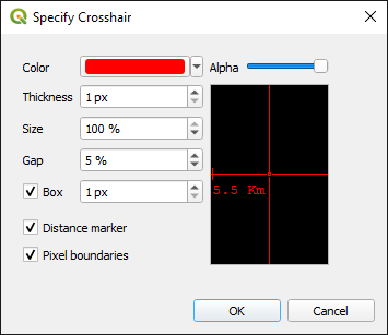
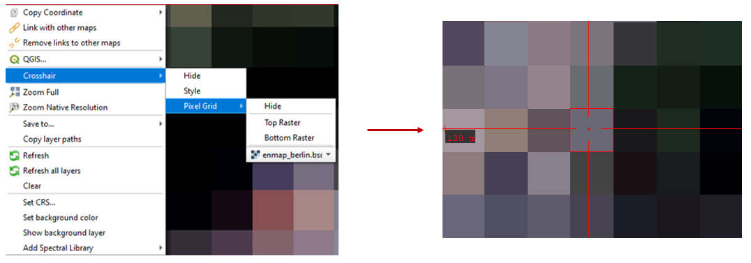
First activate the crosshair for the respective image. Click with the right mouse button in the image. Select Crosshair > Pixel Grid > desired raster image.
Now you should see a red square around your pixel and a red dot indicating the position of the pixel profile.
To identify, select and add a pixel profile, use the following key combinations:
Shortcut
Action
←/↑/↓/→
Move the map
Ctrl + ←/↑/↓/→
Select next pixel in arrow direction
Ctrl + S
Add the selected pixel profile candidate
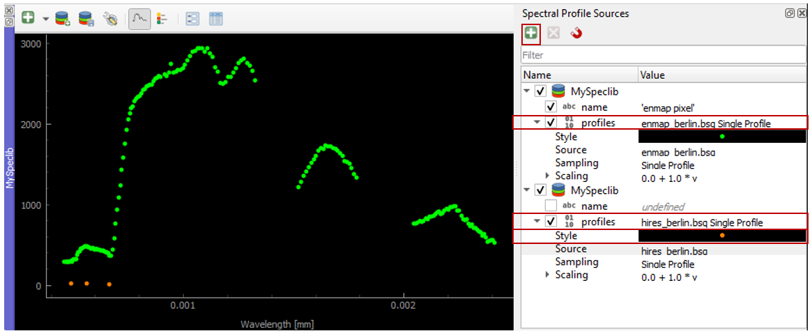
Add profiles from another raster image
Sometimes, you want to compare spectral profiles from different raster sources. The Spectral Profile Source panel allows you to change the default settings of the
Identify tool so that you can select profiles from different images at the same time.
If the Spectral Profile Source Panel is not already visible, open it via View ‣ Panels ‣ Spectral Profile Sources.
Add another profile source relation with and change the Source to the desired raster images.
If you now collect new spectral information, two profiles will appear in the same Spectral Library Window.
Tip
Change the color of one of the profile by changing the Style in the Spectral Profile Sources.
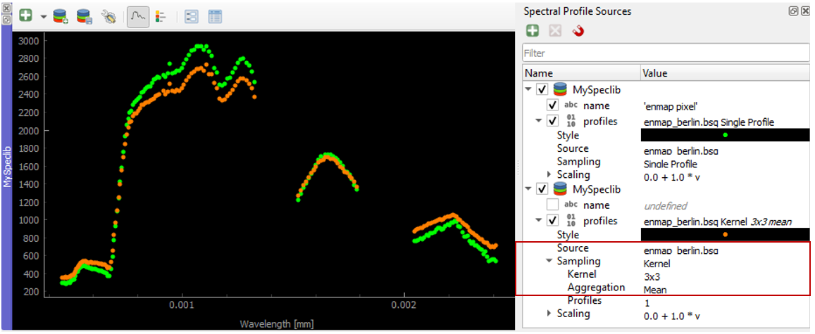
In a similar way you can compare profiles from the same raster image but using a different sampling methods.
In the second relation set the Source to the same image as the first relation.
Change the Sampling to e.g. a 3x3 Kernel mean profile.
You can also add more information to your spectral library by using the attribute table.
Add additional fields to the table, e.g. in order to add information to every spectrum (id, name, classification label, …).
Activate the Table view and enable the Editing mode.
Now you can use the Add Field dialog to add a new column.
Select a data type of your choice.
A new column is added to the attribute table, which you can edit with a double click.
To delete a column, use the Delete field button.
Tip
When you add a new attribute to the table, you can also choose to use it to store new spectral profiles by checking the Use to store spectral profiles checkbox. String, text and binary format can be used to store spectral profiles.
Add information in the layer properties window
It is also possible to add new information to the attribute table in the Layer Properties of the Spectral Library.
Click on to open the spectral library properties.
Navigate to the Fields tab and add a new field. Note: This view does not allow you to set the option Use to store spectral profiles.
Overview of the Layer Properties / Fields section
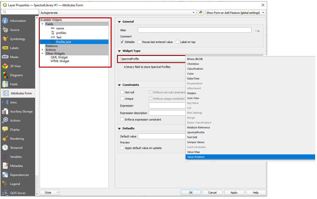
In addition, the Layer Properties panel allows you to set a certain widget for a specific column.
Switch to the Attributes Form tab in the Layer Properties, select the desired column and choose a certain widget type, e.g. a default range, color, spectral profiles etc.
Selecting widget types for specific columns
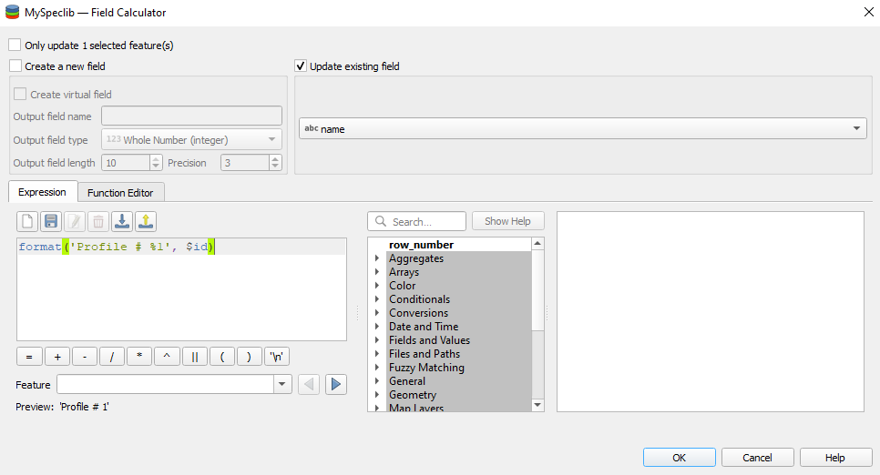
The field calculator
The field calculator allows you to modify or assess spectra and calculate new columns or modify existing ones using an expression.
Overview of the Field Calculator
Selecting spectra
Spectra can be selected in the attribute table and in the plot window itself. Selected spectra will be highlighted (blue background in the table; thicker line in a different color in the plot window).
Hold the Shift key to select multiple spectra.
A selection can be removed by clicking the button.
Selected spectra can be removed by using the button.
Tip
You can inspect an individual value of a spectrum by holding the Alt key and clicking some position along the spectrum
It is also possible to select and filter profiles with the common vector filter and selection tools, e.g. select spectra by expression:
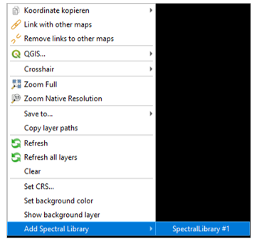
Locations of spectra (if available) can be visualized as a point layer by right-clicking into the map window, and selecting Add Spectral Library > SpectralLibrary #
Create / Modify profiles with the Field Calculator
As already mentioned, the Field Calculator can modify attribute values of all or selected features.
In addition, the field calculator can be used to calculate spectral profiles.
Create a new Spectral Profile field based with Add Field, use string, text or binary format and tick the Ise to store Spectral Profiles box.
Open the field calculator and search for spectralData or spectralMath in the Spectral Libraries tab.
SpectralMath allows you to modify spectral profiles with Python code.
To use the SpectralMath function, select a field from which to take the spectral profiles, define an expression and the format.
spectralMath("<profile field 1>",...,"<profile field n>",'<python code>','<output format>')
Note: The last argument defines the output format. It must correspond to the type you assigned when creating the new column.
Example of calculating new spectral profiles
SpectralData returns spectral profile values.
The following table shows some examples of how spectralMath and spectralData can be used.
Description
Example
Multiply the existing profiles
spectralMath(“profiles”, ‘y *=2’, ‘text’)
Create a new profile with x and y values
spectralMath(‘x,y=[1,2,3],[20,30,25]’)
Return spectral profile values from map with spectral data from spectral profiles in field column “profiles”
spectralData(“profiles”)
Return xUnit string of the spectral profile e.g. ‘nm’ for wavelength unit
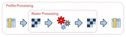
The Spectral Processing framework allows you to use raster processing algorithms to create new profiles.
Field values of your spectral library will be converted into artificial one-line raster images. In principally, this can be done with most of the field types:
Field Type
Raster Size (band, height, n)
type
Spectral Profile
nb, 1, n
int/float
integer
1, 1, n
integer
float
1, 1, n
float
text
1, 1, n
int (classification)
These temporary raster images are input to standard QGIS processing algorithms or QGIS processing models.
If they generate raster outputs, these outputs can be converted back into field values of the spectral library:
Raster Output
Spectral library Field Type
(>1, 1, n) int/float
Spectral Profile
(1, 1, n) int
integer
(1, 1, n) float
float
This allows you to use the same algorithms to modify spectral profiles as you may want to use to manipulate raster images.
Furthermore, you can make use the QGIS model builder to create (potentially very large and complex) models and use them for both,
spectral libraries and raster image processing.
To use the Spectral Processing tool open and choose the desired algorithm, e.g. Spectral resampling.
Select the input profiles to be translated to the temporary raster layer and specify the outputs. Select an existing field or enter a name to create a new field.
The Profile Plot displays spectral profiles. Toggling the Profile View icon shows or hides the plot panel.
This can be useful, for example to enlarge the attribute table and focus on attribute modifications.
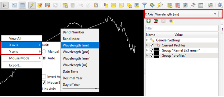
You can adjust the extent of the visualized data range and units
in the plot context menu
using the mouse cursor while keeping the right mouse button pressed
in the visualization settings view
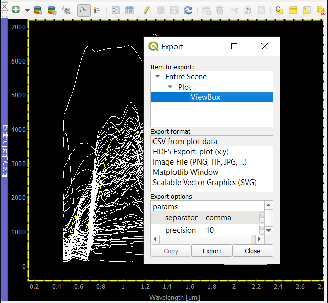
You can also export the entire plot scene or visible view box by clicking into the plot and select Export.
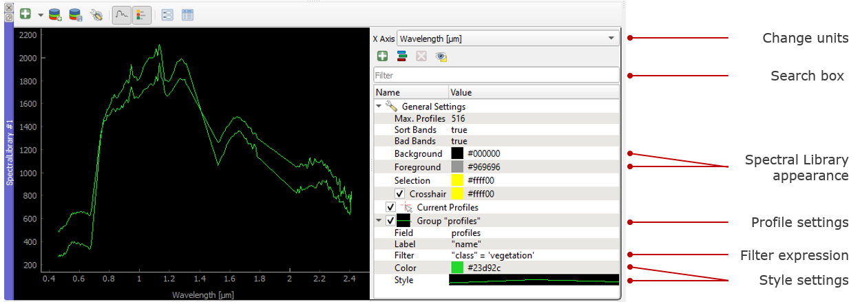
The visualization settings of the spectral library allow you to customize the view according to your needs.
You can define multiple visualization groups that describe how profiles from a specific field and with specific attributes should be visualized.
Overview of the visualization settings in the Spectral Library window
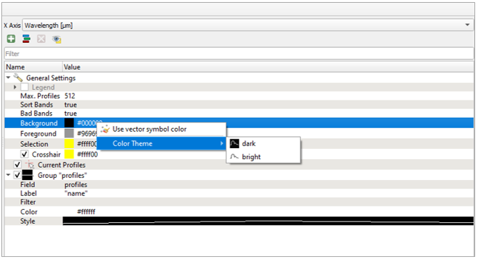
It is also possible, to change the appearance of the Spectral Library window, i.e., bright or dark.
Moreover, activate or deactivate the crosshair and choose a color.
The Current Profiles section shows you all the spectra that have been collected but do not yet appear in the attribute table. Change the color and symbol, or add a line between the points by double clicking the profile below the Current Profile section and adjust the style settings.
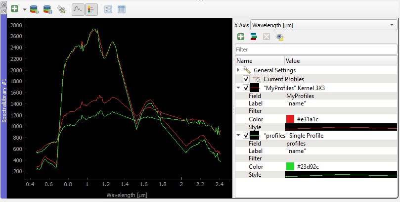
Working with multiple visualization groups
The spectral library visualization settings also allow you to add several profile Groups with different style settings.
Add a second visualization group with .
If you want rename Group “profiles”.
Change the color for both groups in the Color.
Under Field you can specify which spectral profile column of the attribute table you want to use.
If you have more than one column that stores spectral information, you can have different visualization groups using different profiles.
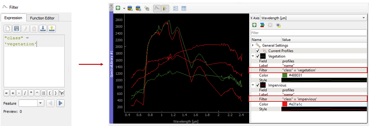
If you have only one column where spectral information is stored, but you have another column storing e.g. class names,
you can use the Filter field to define an expression and select only specific class names, e.g. Impervious and Vegetation and visualize these profiles in different colors.
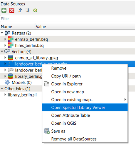
Loading or Saving a spectral library means to load or save vector files.
Load any vector source in the Data Source Panel into a Spectral Library Viewer.
The vector layer does not need to contain any Spectral Profile fields. You can add or define them afterwards.
If your spectral library uses an in-memory vector layer backend, all data will be lost if the layer is closed.
This is the case if the Spectral Library Viewer was opened from scratch with an empty spectral library.
In this case, don’t forget to export collected profiles before closing the Spectral Library Viewer.
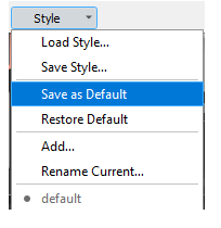
If your spectral library already uses a file backend (e.g. .gpkg, .geojson), Style and other layer specific information
are not saved in the data source file, but the QGIS project or a QGIS specific sidecar .qml file.
Open Layer properties > Symbology > Style > Save Default to create or update the .qml file and ensure that the Spectral Profile fields will be restored when re-opening the data set.
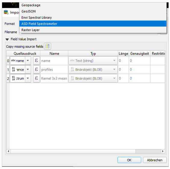
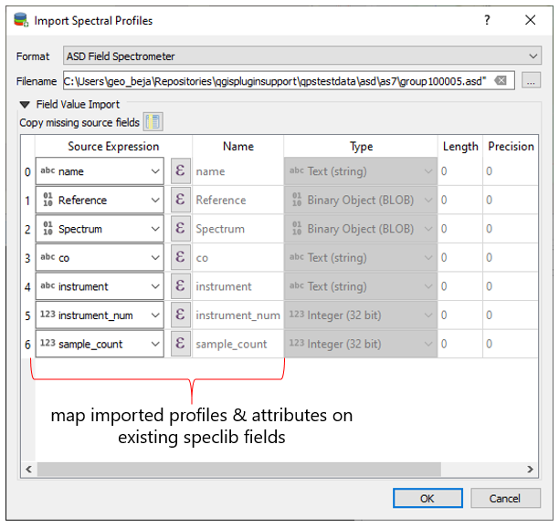
The Export dialog allows you to export all or selected profiles as Geopackage (.gpkg), GeoJSON (.geoson) or ENVI Spectral Library (.sli).
The ENVI Spectral Library does not allow saving profiles with different spectral settings (number of bands, wavelength units, FWHM, …)
in the same file. Therefore, you need to select one (out of multiple) profile fields.
Profiles with different spectral settings will be exported into different ENVI files.
The EnMAP-Box stores the minimum data to plot a single profile in a JSON object. In its most simple way, this JSON object
contains a single array “y” of length n, with n = number of spectral profile values:
{"y":[43,23,45,63,45]}
In this case it can be assumed that the corresponding ‘x’ values are an increasing band index “x”: [0, 1, 2, 3, 4].
The JSON object can describe the “x”, the axis units and a vector of bad band values explicitly:
Member
Content
y
An array with n profile values
x
An array with n profile value locations
yUnit
String that describes the unit of y values
xUnit
String that describes the x value unit
bbl
A bad band list
Other metadata to describe spectra profiles are stored in additional vector layer fields.
As JSON object, a single hyperspectral EnMAP profile may therefore look like:
 on the toolbar and check or uncheck the desired
toolbar.
on the toolbar and check or uncheck the desired
toolbar.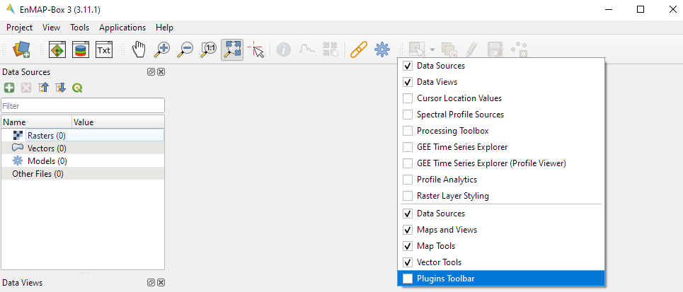


 Raster Data
 for default raster layers (continuous value range)
 for mask raster layers
 for classification raster layers
 Vector Data
 Spectral Libraries
 Models


 Synchronize Data Sources with QGIS
button. Now they should appear in the data source panel and can be added to a Map View.
Synchronize Data Sources with QGIS
button. Now they should appear in the data source panel and can be added to a Map View.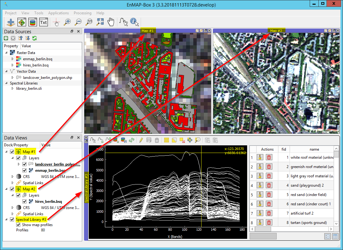
 selects profiles from the top-most raster layer by default. The Profile Source panel allows to change this behaviour
and to control:
selects profiles from the top-most raster layer by default. The Profile Source panel allows to change this behaviour
and to control: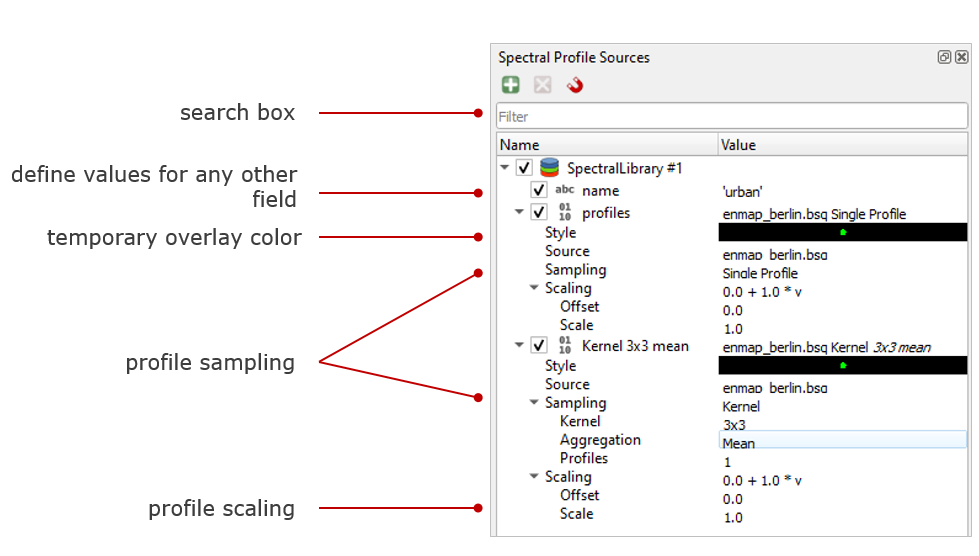

 Identify cursor location value option activated and click somewhere in the map view.
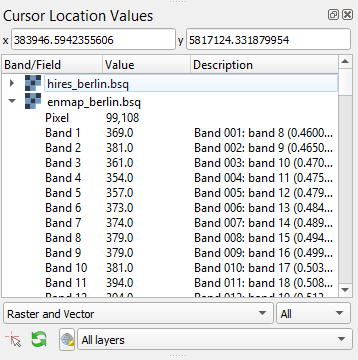
 Select CRS button (e.g. for switching to lat/long coordinates).
 Open a Map View button. Once you added a
Map View, it will be listed in the
Open a Map View button. Once you added a
Map View, it will be listed in the 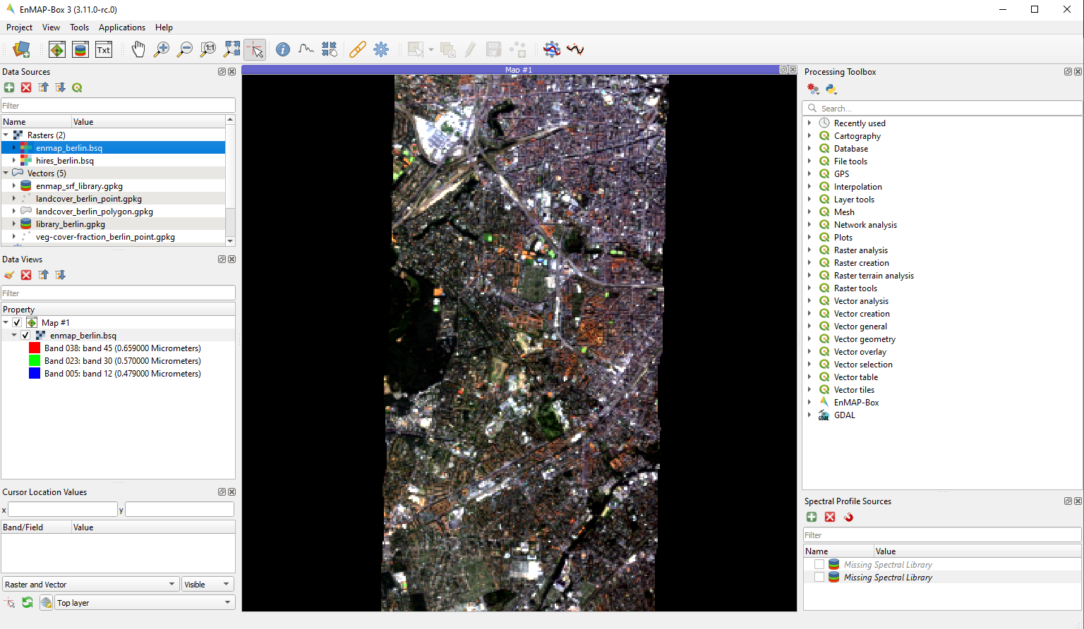
 Link map scale and center
 Link map scale
 Link map center
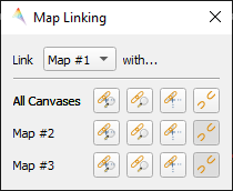
 .
.
 button in the toolbar or open a new window from the menu .
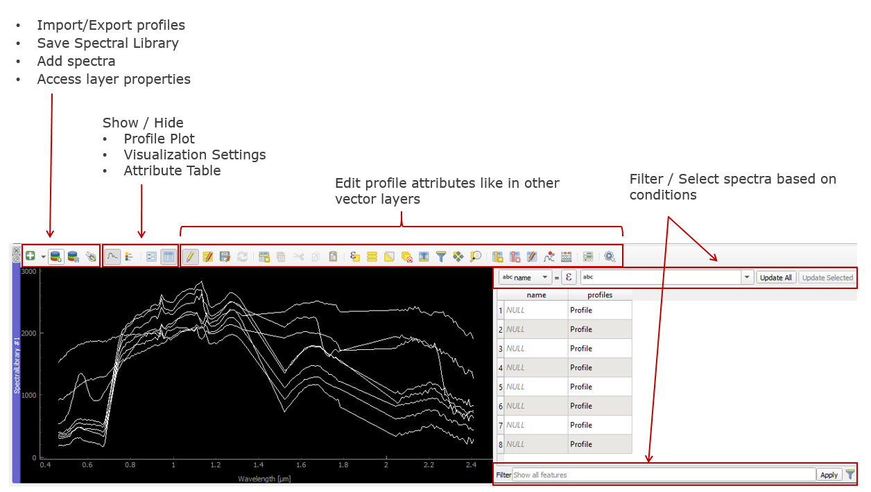


 and
and 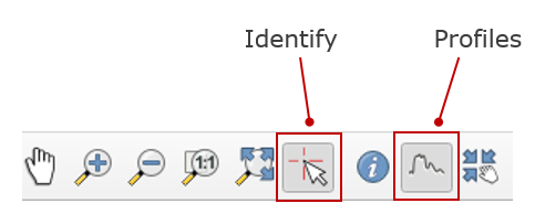
 to keep the candidate profile in the spectral library. Activate Add profiles automatically
  to collect multiple profiles and display them all in the same spectral library.
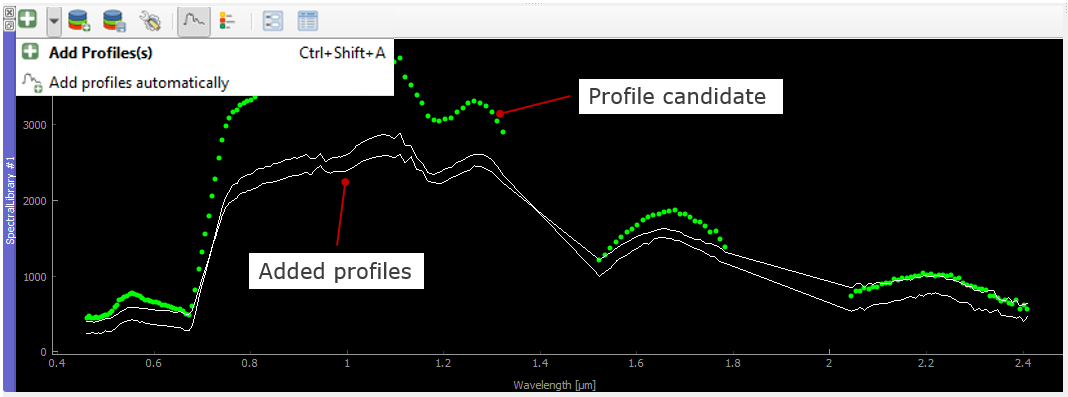
 and enable the Editing mode
  .
. dialog to add a new column.
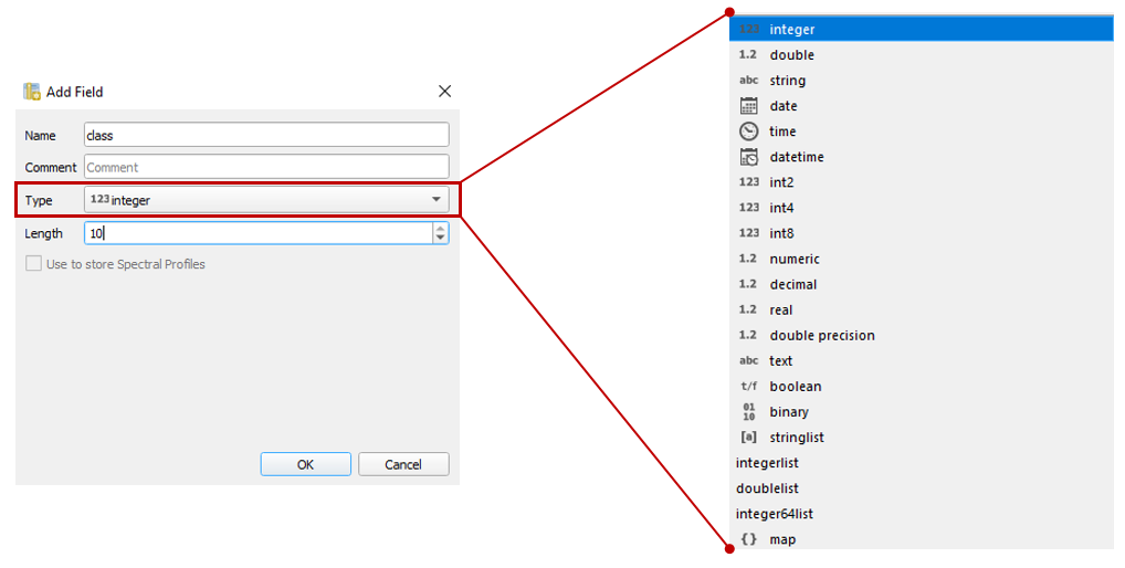
 .
. to open the spectral library properties.
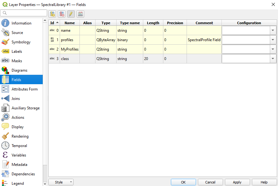
 button.
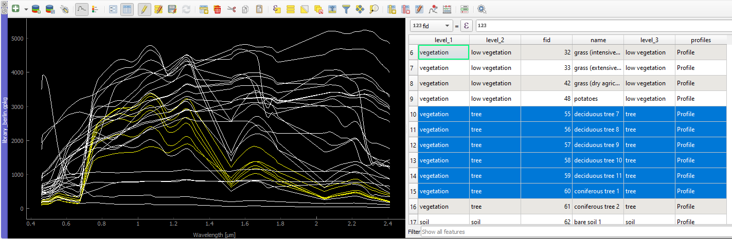
 button.
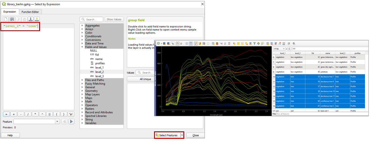
 and search for spectralData or spectralMath in the Spectral Libraries tab.
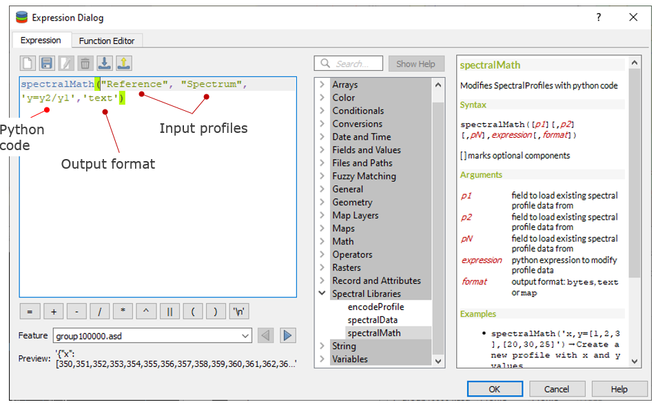
 and choose the desired algorithm, e.g. Spectral resampling.
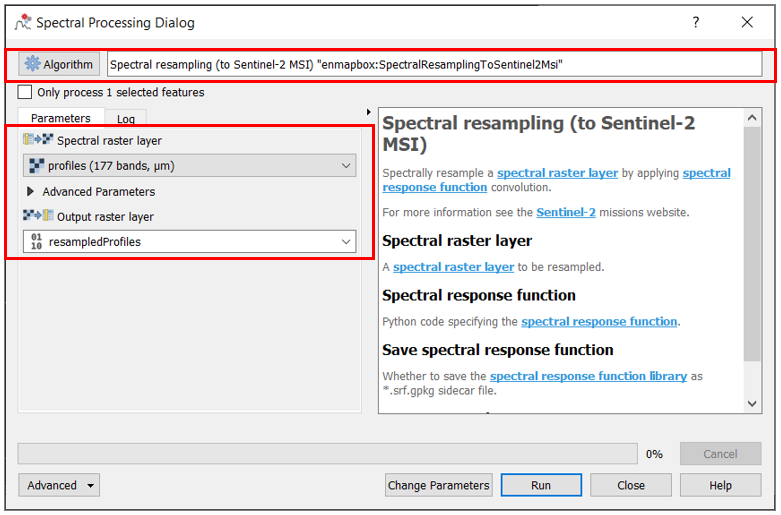
 tab and select the Categorized renderer at the top.
 button.
 .
.
 allows you to export all or selected profiles as Geopackage (.gpkg), GeoJSON (.geoson) or ENVI Spectral Library (.sli).
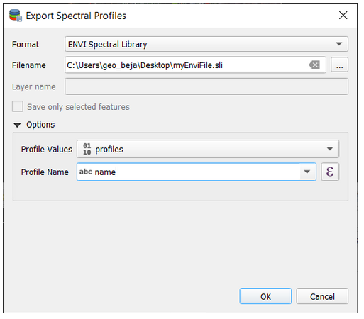
 button.