Using Raster math for performing both simple and complex raster arithmetics
Raster math is a powerful raster calculator inspired by the QGIS Raster calculator, the GDAL Raster calculator and ENVI Band Math. In addition to those tools, Raster math supports multi-band arrays, vector layer inputs, multi-line code snippets and metadata handling.
As a getting started, we load the EnMAP-Box testdata, open Raster math under , load and execute the predefined NDVI code snippet:

Using simple expressions
Now we can use the Available data sources and the Operators buttons to quickly define an expression. Let’s just mask the enmap_berlin raster layer with the landcover_berlin_polygon vector layer.
In this expression, the enmap_berlin variable is a 3d numpy array with shape [177 bands, ysize, xsize] and landcover_berlin_polygon is a binary 0/1-valued rasterization of the vector geometries, also given as a 3d numpy array with shape [1 band, ysize, xsize].
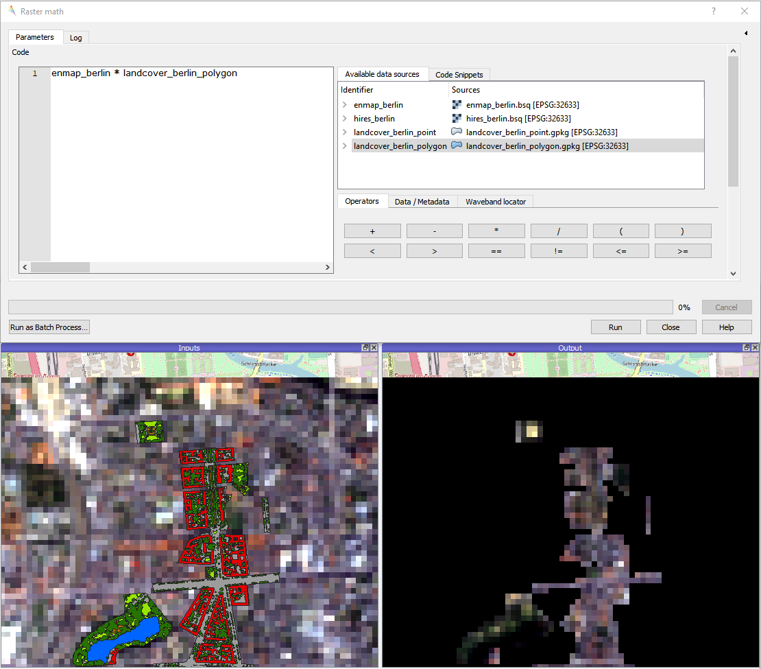
Note that the output raster is correctly masked, but we haven’t set an appropriate no data value, nor have we taken care of wavelength information or any other source metadata.
Using multi-line code snippets and handle metadata
To enable more complex computations and metadata handling, we can use multi-line code snippets.
Let’s advance on the simple expression from above and improve it, by setting a no data value, and proper metadata handling.
Use the Available data sources and the Data / Metadata buttons to quickly define the code snippet.

Using individual bands by band index, band position or wavelength location
When using a raster layer inside a calculation, the default is to read all bands into memory. This can be really disadvantageous in case you only need two bands to calculate the NDVI.
For example, you can index into the enmap_berlin array to access the red and nir band:
# find bands
red = enmap_berlin[36]  # band 37 at 653 Nanometers
nir = enmap_berlin[65]  # band 66 at 864 Nanometers

# calculate NDVI
ndvi = (nir - red) / nir + red
But it would be more efficient to access those bands via the special @<band number> syntax.
This way, only two bands are mapped into memory as individual arrays of shape [1 band, ysize, xsize]:
red = enmap_berlin@37
nir = enmap_berlin@66
In case of a spectral raster layer, bands can also be accessed via a target wavelength in Nanometers:
red = enmap_berlin@655nm
nir = enmap_berlin@865nm
You may use the Waveband locator for quickly selecting some predefined sensor waveband locations:

Using band masks
ToDo
Using advanced band subsetting
ToDo
Using special variables and logging feedback
ToDo
Running Raster math from command line
Like any other processing algorithm, Raster math can be executed from the command line. Here is a simple NDVI example:
- Anaconda Prompt:
Activate your QGIS conda environment and use the qgis_process command line tool:
qgis_process run enmapbox:RasterMath -- code="(R1@865nm - R1@655nm) / (R1@865nm + R1@655nm)" R1=enmap_berlin.bsq outputRaster=c:/result/ndvi.tif
- OSGeo4W Shell:
As an initial step, run qgis_process-qgis.bat to setup the environment. Now use the qgis_process command line tool:
qgis_process run enmapbox:RasterMath -- code="(R1@865nm - R1@655nm) / (R1@865nm + R1@655nm)" R1=enmap_berlin.bsq outputRaster=c:/result/ndvi.tif