1. Implementing Processing Algorithms
Overview
In this tutorial will you learn:
how to implement an image processing algorithm in Python (i.e. core algorithm) using the HUB Datacube API
how to integrate the core algorithm into the QGIS Processing Framework (i.e. processing algorithm)
how to integrate the processing algorithm into the EnMAP-Box (i.e. EnMAP-Box Application)
To put everything into context, we will follow the use case described below.
Use case description
In this tutorial we want to implement a workflow for regression-based landcover fraction unmixing. We use the EnMAP-Box testdata to explain and visualize all the details, but the implementation is not limited to that specific dataset.
Our data are a simulated 30 m EnMAP raster and a vector with detailed landcover polygons:
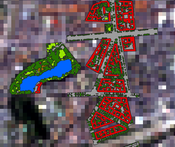
Fig. 47 Simulated 30 m EnMAP raster (enmap_berlin.bsq) overlayed by landcover polygons (landcover_berlin_polygon.shp)
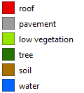
Fig. 48 Landcover categories
The landcover is rasterized at a detailed resolution (e.g. 10 times finer than the EnMAP resolution):
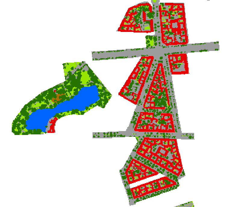
Fig. 49 Rasterized landcover at 3 m resolution (oversampling the EnMAP resolution by factor 10)
The rasterized landcover is aggregated into the target resolution (i.e. 30 m EnMAP):
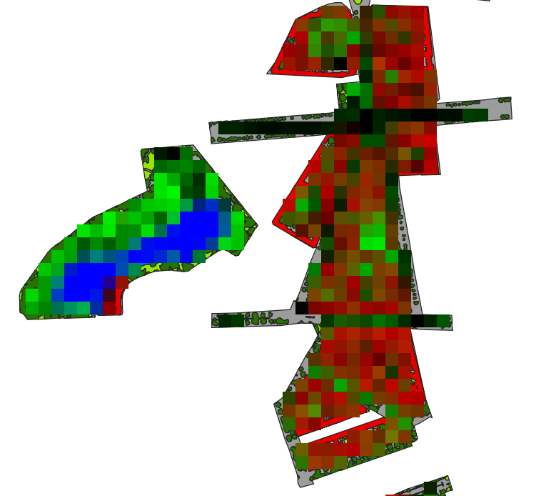
Fig. 50 Aggregated 30 m landcover fraction as false-color-composition: Red=’roof’, Green=’tree’ and Blue=’water’
Finally, a Random Forest Regressor is fitted with the created dataset and applied to the whole EnMAP raster to derive a landcover fraction map:
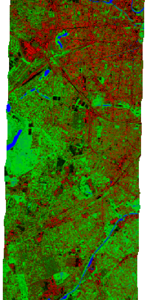
Fig. 51 Predicted 30 m landcover fractions as false-color-composition: Red=’roof’, Green=’tree’ and Blue=’water’
Core algorithm implementation
The core algorithm is implemented using the HUB Datacube API. Here is a full listing:
Code listing
# 0
from _classic.hubdc.core import *
# 1
def regressionBasedUnmixing(filename, rasterFilename, vectorFilename, classAttribute,
                            oversampling=10, coverage=0.9, n_estimators=100):
    '''
    This function derives landcover pixel fractions from the given raster and vector maps,
    fits a random forest regressor to that dataset and applies it the the raster predicting
    (multi-band) landcover fractions and stores it at the given ``filename``.

    :param filename: output fraction raster filename
    :param rasterFilename: input raster filename
    :param vectorFilename: input vector filename
    :param classAttribute: attribute with class ids (values 1 to number of classes)
    :param oversampling: oversampling factor defines how accurate the landcover polygons
                         are aggregated into pixel fractions
    :param coverage: threshold between 0 and 1 that defines the minimal coverage a pixel
                     must have to be concidered as training sample.
    :param n_estimators: number of trees used for the random forest regressor
    '''

# 2
    #  open datasets
    raster = openRasterDataset(filename=rasterFilename)
    vector = openVectorDataset(filename=vectorFilename)
# 3
    # rasterize landcover polygons into classes (detailed resolution)
    grid = raster.grid()
    gridOversampled = Grid(extent=grid.extent(), resolution=grid.resolution() / oversampling)
    idRaster = vector.rasterize(grid=gridOversampled, burnAttribute=classAttribute, initValue=0)
    idArray = idRaster.array()
# 4a
    # aggregate classes into class cover fractions (target resolution)
    numberOfClasses = int(np.max(idArray))
    ysize, xsize = grid.shape()
    fractionArray = np.empty(shape=(numberOfClasses, ysize, xsize), dtype=np.float32)
# 4b
    for id in range(1, numberOfClasses+1):

        # create class occurrence mask
        maskArray = np.float32(idArray == id)
        maskRaster = RasterDataset.fromArray(array=maskArray, grid=gridOversampled)
# 4c
        # aggregate occurrences into fractions
        fractionRaster = maskRaster.translate(grid=grid, resampleAlg=gdal.GRA_Average)
        fractionArray[id-1] = fractionRaster.array()
# 5
    # calculate pixel coverage
    coverageArray = np.sum(fractionArray, axis=0)
# 6
    # draw all samples that satisfy the minimal coverage condition
    valid = coverageArray >= coverage
    profiles = raster.array()[:, valid]
    labels = fractionArray[:, valid]
# 7
    # fit a random forest regressor
    from sklearn.ensemble import RandomForestRegressor
    rfr = RandomForestRegressor(n_estimators=n_estimators)
    X = profiles.T
    y = labels.T
    rfr.fit(X=X, y=y)
# 8
    # predict fraction map
    array = raster.array()
    valid = array[0] != raster.noDataValues()[0]
    X = array[:, valid].reshape(raster.zsize(), -1).T
    y = rfr.predict(X=X)
    fractionArray = np.full(shape=(numberOfClasses, ysize, xsize), fill_value=-1., dtype=np.float32)
    fractionArray[:, valid] = y.T
# 9a
    # store as raster and set metadata
    driver = RasterDriver.fromFilename(filename=filename)
    fractionRaster = RasterDataset.fromArray(array=fractionArray, grid=grid, filename=filename, driver=driver)
    fractionRaster.setNoDataValue(value=-1)
# 9b
    # - get class names from attribute definition file (i.e. *.json)
    jsonFilename = join(dirname(vectorFilename), '{}.json'.format(splitext(basename(vectorFilename))[0]))
    if exists(jsonFilename):
        import json
        with open(jsonFilename) as file:
            attributeDefinition = json.load(file)
        for id, name, color in attributeDefinition[classAttribute]['categories']:
            if id == 0:
                continue # skip 'unclassified' class
            fractionRaster.band(index=id-1).setDescription(value=name)
Test environment
Here is a test setup using the EnMAP-Box testdata:
import enmapboxtestdata
from tut1_app1.core import regressionBasedUnmixing

regressionBasedUnmixing(filename='fraction.bsq',
                        rasterFilename=enmapboxtestdata.enmap,
                        vectorFilename=enmapboxtestdata.landcover_polygon,
                        classAttribute='level_3_id')

if True: # show the result in a viewer
    from _classic.hubdc.core import openRasterDataset, MapViewer
    rasterDataset = openRasterDataset(filename='fraction.bsq')
    MapViewer().addLayer(rasterDataset.mapLayer().initMultiBandColorRenderer(0, 3, 5, percent=0)).show()
Task
Start PyCharm via the PyCharm Start Script.
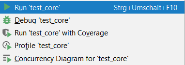
Open and run the test_core.py script (right click into the editor and click Run ‘test_core’).
The final result will be shown in a map viewer:
Code discussion
In the following section we will explore the implementation interactively and in great detail.
Task
Open the core.py module.
Set breakpoints at the beginning of each section, e.g.
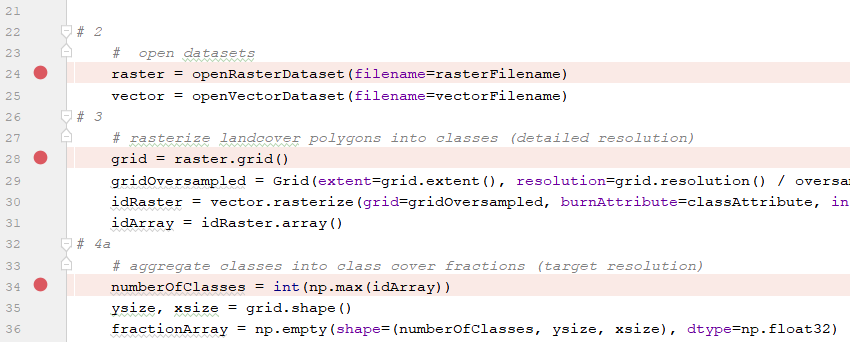
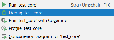
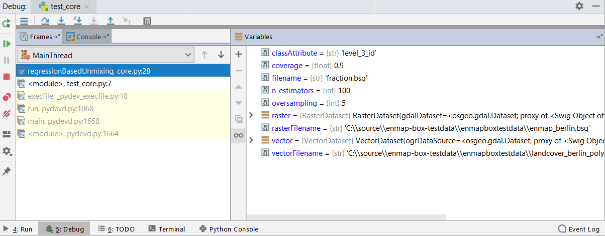
Run the test_core.py script in debug mode.
Investigate the program state at each breakpoint via the debug view.
Answer the questions stated below.
Import everything from the hubdc.core module:
from _classic.hubdc.core import *
Define the core function signature and provide a descriptive doc string:
def regressionBasedUnmixing(filename, rasterFilename, vectorFilename, classAttribute,
                            oversampling=10, coverage=0.9, n_estimators=100):
    '''
    This function derives landcover pixel fractions from the given raster and vector maps,
    fits a random forest regressor to that dataset and applies it the the raster predicting
    (multi-band) landcover fractions and stores it at the given ``filename``.

    :param filename: output fraction raster filename
    :param rasterFilename: input raster filename
    :param vectorFilename: input vector filename
    :param classAttribute: attribute with class ids (values 1 to number of classes)
    :param oversampling: oversampling factor defines how accurate the landcover polygons
                         are aggregated into pixel fractions
    :param coverage: threshold between 0 and 1 that defines the minimal coverage a pixel
                     must have to be concidered as training sample.
    :param n_estimators: number of trees used for the random forest regressor
    '''
Open the raster and vector input files.
    #  open datasets
    raster = openRasterDataset(filename=rasterFilename)
    vector = openVectorDataset(filename=vectorFilename)
Exercise
Investigate the raster and vector variables via the Evaluate View (press Alt+F8).
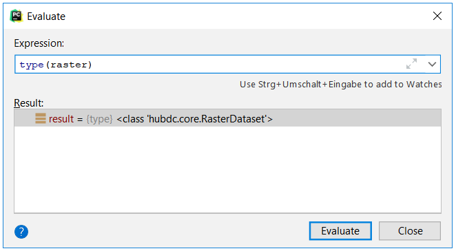
1. What are their types?
The type of raster is hubdc.core.RasterDataset.
The type of vector is hubdc.core.VectorDataset.
2. Find more information in the HUB Datacube Documentation!
Usage examples are listed in the Cookbook:RasterDataset recipes
VectorDataset recipes
3. What is the shape (i.e. bands, ysize, xsize) of the raster?
raster.shape() = bands, ysize, xsize = (177, 400, 220)
Get the target grid from the raster and define a new gridOversampled with the same extent,
but finer oversampled resolution.
Create a class idRaster by rasterizing the vector class attribute into the oversampled grid.
Read the data from the id raster into a Numpy idArray.
Note
It is assumed that the id of the first class is 1, of the second class is 2, and so on. The largest id is equal to the number of classes.
    # rasterize landcover polygons into classes (detailed resolution)
    grid = raster.grid()
    gridOversampled = Grid(extent=grid.extent(), resolution=grid.resolution() / oversampling)
    idRaster = vector.rasterize(grid=gridOversampled, burnAttribute=classAttribute, initValue=0)
    idArray = idRaster.array()
Exercise
1. Explain by what elements a grid is characterized!
A grid is characterized by an Extent (bounding box and projection) and a Resolution.
2. What is the difference between grid and gridOversampled.
The resolution, and derived from that, their shape:grid.shape() = ysize, xsize = (400, 220)
gridOversampled.shape() = ysize, xsize = (4000, 2200)
3. What is the shape of the idArray and what values are stored in it?
idArray.shape = bands, ysize, xsize = (1, 4000, 2200)
np.unique(idArray) = [0, 1, 2, 3, 4, 5, 6]
Derive the number of classes fom the idArray and initialize the fractionArray.
    # aggregate classes into class cover fractions (target resolution)
    numberOfClasses = int(np.max(idArray))
    ysize, xsize = grid.shape()
    fractionArray = np.empty(shape=(numberOfClasses, ysize, xsize), dtype=np.float32)
Exercise
What is the shape of the fractionArray?
fractionArray.shape = bands, ysize, xsize = (6, 400, 220)
Derive for each class a binary occurrence maskArray and create a maskRaster from it.
    for id in range(1, numberOfClasses+1):

        # create class occurrence mask
        maskArray = np.float32(idArray == id)
        maskRaster = RasterDataset.fromArray(array=maskArray, grid=gridOversampled)
Exercise
Visualize the maskRaster in a map viewer!
MapViewer().addLayer(maskRaster.mapLayer()).show()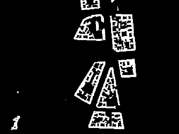
Aggregate the maskRaster into the fractionRaster by resampling it into the target gridOversampled.
Read the data from the fractionRaster into the prepared fractionArray.
        # aggregate occurrences into fractions
        fractionRaster = maskRaster.translate(grid=grid, resampleAlg=gdal.GRA_Average)
        fractionArray[id-1] = fractionRaster.array()
Exercise
Visualize the fractionRaster in a map viewer!
MapViewer().addLayer(fractionRaster.mapLayer()).show()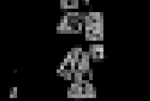
Sum up all class-wise fractions into an overall pixel coverageArray.
    # calculate pixel coverage
    coverageArray = np.sum(fractionArray, axis=0)
Compare the overall coverageArray to the minimal coverage threshold to find sufficiently covered pixel.
For all valid pixels, extract the raster profiles and class fraction labels.
    # draw all samples that satisfy the minimal coverage condition
    valid = coverageArray >= coverage
    profiles = raster.array()[:, valid]
    labels = fractionArray[:, valid]
Exercise
How many valid pixel are left?
np.sum(valid) = 1666If the coverage condition would be 0.5, how many valid pixel are left?
np.sum(coverageArray >= 0.5) = 2038What are the shapes of the profiles and labels?
profiles.shape = bands, samples = 177, 1666labels.shape = bands, samples = 6, 1666Tip
Numpy array indexing can become quite complex. Get yourself familiarized with it.
Use the extracted profiles and labels to fit a multi-target Random Forest Regressor.
    # fit a random forest regressor
    from sklearn.ensemble import RandomForestRegressor
    rfr = RandomForestRegressor(n_estimators=n_estimators)
    X = profiles.T
    y = labels.T
    rfr.fit(X=X, y=y)
Tip
Get yourself familiarized with the Scikit-Learn RandomForestRegressor.
Exercise
Plot the Random Forest feature importances! Use the plt.plot function.
plt.plot(rfr.feature_importances_)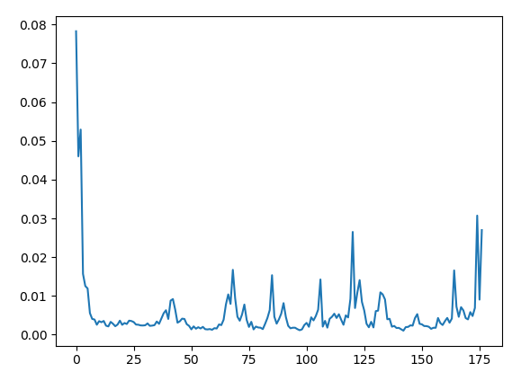
Read raster data into an array.
Identify all valid pixels.
Extract and prepare valid samples as input X for prediction.
Predict class fractions y using the Random Forest Regressor for all valid pixels.
Initialize result fractionArray with a no data value of -1.
Fill prediction y into the fractionArray.
    # predict fraction map
    array = raster.array()
    valid = array[0] != raster.noDataValues()[0]
    X = array[:, valid].reshape(raster.zsize(), -1).T
    y = rfr.predict(X=X)
    fractionArray = np.full(shape=(numberOfClasses, ysize, xsize), fill_value=-1., dtype=np.float32)
    fractionArray[:, valid] = y.T
Exercise
The way the valid pixel mask is calculated, is not universal. What is the problem and how could it be improved?
We only evaluate the first band for no data pixel. If the value of a pixel in the first band is valid, but has a no data value in one of the other bands, we would pass an invalid sample to the predict method, which could cause problems.Solution:
valid = np.all([a != ndv for a, ndv in zip(array, raster.noDataValues()], axis=0)Write the fractionArray as a fractionRaster and set the no data value.
    # store as raster and set metadata
    driver = RasterDriver.fromFilename(filename=filename)
    fractionRaster = RasterDataset.fromArray(array=fractionArray, grid=grid, filename=filename, driver=driver)
    fractionRaster.setNoDataValue(value=-1)
Exercise
What raster format was used for creating the fractionRaster?
We derive the raster driver from the output filename extention '.bsq', which is associated with the ENVI driver.Investigate the RasterDriver.fromFilename source for more details.
How would you create a GeoTiff output?
Change the output filename to 'fraction.tif'.Or set the driver explicitely:
driver = RasterDriver(name='GTiff')
Tip
Get yourself familiarized with the full list of GDAL Raster Formats.
Tip
The EnMAP-Box has introduced a special attribute definition format for categorical vector data, stored as a JSON file. It allows to specify category names and colors:
{
  "level_1_id": {
    "categories":  [
      [0, "unclassified", [0, 0, 0]],
      [1, "impervious", [230, 0, 0]],
      [2, "vegetation", [56, 168, 0]],
      [3, "soil", [168, 112, 0]],
      [4, "water", [0,100,255]]
    ],
    "no data value": 0,
    "description": "Classification"
  },
  "level_2_id": {
    "categories":  [
      [0, "unclassified", [0, 0, 0]],
      [1, "impervious", [230, 0, 0]],
      [2, "low vegetation", [152, 230, 0]],
      [3, "tree", [38, 115, 0]],
      [4, "soil", [168, 112, 0]],
      [5, "water", [0,100,255]]
    ],
    "no data value": 0,
    "description": "Classification"
  },
  "level_3_id": {
    "categories":  [
      [0, "unclassified", [0, 0, 0]],
      [1, "roof", [230, 0, 0]],
      [2, "pavement", [156, 156, 156]],
      [3, "low vegetation", [152, 230, 0]],
      [4, "tree", [38, 115, 0]],
      [5, "soil", [168, 112, 0]],
      [6, "water", [0,100,255]]
    ],
    "no data value": 0,
    "description": "Classification"
  }
}
The category legend for the level_3_id attribute would look like this.
If an attribute definition file is available, set the category names as raster band names.
    # - get class names from attribute definition file (i.e. *.json)
    jsonFilename = join(dirname(vectorFilename), '{}.json'.format(splitext(basename(vectorFilename))[0]))
    if exists(jsonFilename):
        import json
        with open(jsonFilename) as file:
            attributeDefinition = json.load(file)
        for id, name, color in attributeDefinition[classAttribute]['categories']:
            if id == 0:
                continue # skip 'unclassified' class
            fractionRaster.band(index=id-1).setDescription(value=name)
This concludes the code discussion.
Core algorithm (advanced)
The above core algorithm implementation is operating on the full dataset at once. This may be acceptable for quick and dirty prototyping, small datasets or “throw-away-after-creating-my-results” scenarios.
But if you want to release an algorithm to a wider community, you should consider a more memory-efficient implementation.
Here is an adoption of the original core algorithm, where the data input and output is done on smaller memory-efficient subgrids.
from _classic.hubdc.core import *

def regressionBasedUnmixing(filename, rasterFilename, vectorFilename, classAttribute,
                            oversampling=10, coverage=0.9, n_estimators=100,
                            blockSize=256):
    #  open datasets
    raster = openRasterDataset(filename=rasterFilename)
    vector = openVectorDataset(filename=vectorFilename)

    numberOfClasses = int(np.max([feature.value(attribute=classAttribute) for feature in vector.features()]))

    profiles = list()
    labels = list()
    for subgrid, i, iy, ix in raster.grid().subgrids(size=blockSize):

        # rasterize landcover polygons into classes (detailed resolution)
        gridOversampled = Grid(extent=subgrid.extent(), resolution=subgrid.resolution() / oversampling)
        idRaster = vector.rasterize(grid=gridOversampled, burnAttribute=classAttribute, initValue=0)
        idArray = idRaster.array()

        # aggregate classes into class cover fractions (target resolution)
        ysize, xsize = subgrid.shape()
        fractionArray = np.empty(shape=(numberOfClasses, ysize, xsize), dtype=np.float32)

        for id in range(1, numberOfClasses+1):

            # create class occurrence mask
            maskArray = np.float32(idArray == id)
            maskRaster = RasterDataset.fromArray(array=maskArray, grid=gridOversampled)

            # aggregate occurrences into fractions
            fractionRaster = maskRaster.translate(grid=subgrid, resampleAlg=gdal.GRA_Average)
            fractionArray[id-1] = fractionRaster.array()

        # calculate pixel coverage
        coverageArray = np.sum(fractionArray, axis=0)

        # draw all samples that satisfy the minimal coverage condition
        valid = coverageArray >= coverage
        profiles.append(raster.array(grid=subgrid)[:, valid])
        labels.append(fractionArray[:, valid])

    # stack subgrid results togethter
    profiles = np.hstack(profiles)
    labels = np.hstack(labels)

    # fit a random forest regressor
    from sklearn.ensemble import RandomForestRegressor
    rfr = RandomForestRegressor(n_estimators=n_estimators)
    X = profiles.T
    y = labels.T
    rfr.fit(X=X, y=y)

    # init result fraction raster
    driver = RasterDriver.fromFilename(filename=filename)
    fractionRaster = driver.create(grid=raster.grid(), bands=numberOfClasses, filename=filename)

    for subgrid, i, iy, ix in raster.grid().subgrids(size=blockSize):

        # predict subgrid fractions
        array = raster.array(grid=subgrid)
        valid = array[0] != raster.noDataValues()[0]
        X = array[:, valid].reshape(raster.zsize(), -1).T
        y = rfr.predict(X=X)
        ysize, xsize = subgrid.shape()
        fractionArray = np.full(shape=(numberOfClasses, ysize, xsize), fill_value=-1., dtype=np.float32)
        fractionArray[:, valid] = y.T

        # write subgrid fractions
        fractionRaster.writeArray(array=fractionArray, grid=subgrid)

    # set metadata
    fractionRaster.setNoDataValue(value=-1)

    # - get class names from attribute definition file (i.e. *.json)
    jsonFilename = join(dirname(vectorFilename), '{}.json'.format(splitext(basename(vectorFilename))[0]))
    if exists(jsonFilename):
        import json
        with open(jsonFilename) as file:
            attributeDefinition = json.load(file)
        for id, name, color in attributeDefinition[classAttribute]['categories']:
            if id == 0:
                continue # skip 'unclassified' class
            fractionRaster.band(index=id-1).setDescription(value=name)
Processing Framework integration
To integrate the core algorithm into the QGIS Processing Framework, we derive from the QgsProcessingAlgorithm class. This provides us with an auto-generated graphical user interface:
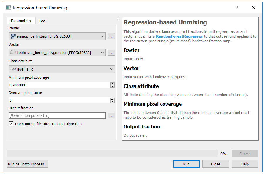
Here is a full listing of the implementation:
Code listing
# 0
from qgis.core import *
from .core import regressionBasedUnmixing

# 1
class RegressionBasedUnmixingProcessingAlgorithm(QgsProcessingAlgorithm):

    P_RASTER = 'inraster'
    P_VECTOR = 'invector'
    P_FIELD = 'field'
    P_COVERAGE = 'coverage'
    P_OVERSAMPLING = 'oversampling'
    P_OUTPUT_FRACTION = 'outfraction'
# 2
    def group(self):
        return 'Workshop'

    def groupId(self):
        return 'workshop' # internal id

    def displayName(self):
        return 'Regression-based Unmixing'

    def name(self):
        return 'RegressionBasedUnmixing' # internal id
# 3
    def initAlgorithm(self, configuration=None):

        # Define required user inputs.
        self.addParameter(QgsProcessingParameterRasterLayer(
            name=self.P_RASTER, description='Raster'))
        self.addParameter(QgsProcessingParameterVectorLayer(
            name=self.P_VECTOR, description='Vector', types=[2])) # polygons only
        self.addParameter(QgsProcessingParameterField(
            name=self.P_FIELD, description='Class attribute', parentLayerParameterName=self.P_VECTOR,
            type=QgsProcessingParameterField.Numeric))
        self.addParameter(QgsProcessingParameterNumber(
            name=self.P_COVERAGE, description='Minimum pixel coverage', type=QgsProcessingParameterNumber.Double,
            defaultValue=0.9, minValue=0, maxValue=1))
        self.addParameter(QgsProcessingParameterNumber(
            name=self.P_OVERSAMPLING, description='Oversampling factor', type=QgsProcessingParameterNumber.Integer,
            defaultValue=5, minValue=0, maxValue=10))
        self.addParameter(QgsProcessingParameterRasterDestination(
            name=self.P_OUTPUT_FRACTION, description='Output fraction'))
# 4
    def processAlgorithm(self, parameters, context, feedback):
        assert isinstance(feedback, QgsProcessingFeedback)

        # try to execute the core algorithm
        try:

            # pass all selected input parameters to the core algorithm
            regressionBasedUnmixing(
                filename=self.parameterAsOutputLayer(parameters, self.P_OUTPUT_FRACTION, context),
                rasterFilename=self.parameterAsRasterLayer(parameters, self.P_RASTER, context).source(),
                vectorFilename=self.parameterAsVectorLayer(parameters, self.P_VECTOR, context).source(),
                classAttribute=self.parameterAsString(parameters, self.P_FIELD, context),
                oversampling=self.parameterAsInt(parameters, self.P_OVERSAMPLING, context),
                coverage=self.parameterAsDouble(parameters, self.P_COVERAGE, context))

            # return all output parameters
            return {self.P_OUTPUT_FRACTION: self.parameterAsOutputLayer(parameters, self.P_OUTPUT_FRACTION, context)}

        # handle any uncatched exceptions
        except:
            # print traceback to console and pass it to the processing feedback object
            import traceback
            traceback.print_exc()
            for line in traceback.format_exc().split('\n'):
                feedback.reportError(line)
            return {}
# 5
    def shortHelpString(self):

        html = '' \
       '<p>This algorithm derives landcover pixel fractions from the given raster and vector maps, fits a ' \
       '<a href="https://scikit-learn.org/stable/modules/generated/sklearn.ensemble.RandomForestRegressor.html">RandomForestRegressor</a> ' \
       'to that dataset and applies it to the the raster, predicting a (multi-class) landcover fraction map.</p>' \
       '<h3>Raster</h3>' \
       '<p>Input raster.</p>' \
       '<h3>Vector</h3>' \
       '<p>Input vector with landcover polygons.</p>' \
       '<h3>Class attribute</h3>' \
       '<p>Attribute defining the class ids (values between 1 and number of classes).</p>' \
       '<h3>Minimam pixel coverage</h3>' \
       '<p>Threshold between 0 and 1 that defines the minimal coverage a pixel must have to be concidered as training sample.</p>' \
       '<h3>Output fraction</h3>' \
       '<p>Output raster.</p>'
        return html
# 6
    def helpUrl(self, *args, **kwargs):
        return 'https://enmap-box.readthedocs.io/'
# 7
    def createInstance(self):
        return type(self)()
Test environment
Here is a test setup using the EnMAP-Box testdata:
from os.path import join, dirname
from qgis.core import QgsProcessingFeedback, QgsApplication
from processing.core.Processing import Processing
from tut1_app1.processingalgorithm import RegressionBasedUnmixingProcessingAlgorithm
import enmapboxtestdata

# init QGIS
qgsApp = QgsApplication([], True)
qgsApp.initQgis()
qgsApp.messageLog().messageReceived.connect(lambda *args: print(args[0]))

# init processing framework
Processing.initialize()

# run algorithm
alg = RegressionBasedUnmixingProcessingAlgorithm()
io = {alg.P_RASTER: enmapboxtestdata.enmap,
      alg.P_VECTOR: enmapboxtestdata.landcover_polygon,
      alg.P_FIELD: 'level_2_id',
      alg.P_COVERAGE: 0.9,
      alg.P_OVERSAMPLING: 10,
      alg.P_OUTPUT_FRACTION: join(dirname(__file__), 'fraction.bsq')}
result = Processing.runAlgorithm(alg, parameters=io)

print(result)

if True: # show the result in a viewer
    from _classic.hubdc.core import MapViewer, openRasterDataset
    fraction = openRasterDataset(filename=result[alg.P_OUTPUT_FRACTION])
    MapViewer().addLayer(fraction.mapLayer().initMultiBandColorRenderer(0, 2, 4, percent=0)).show()
Task
Open and run the test_processingalgorithm.py script in PyCharm.
Prints:
{'outfraction': 'C:/enmap-box-workshop2019/programming_tutorial1/tut1_app1\\fraction.bsq'}
The final result will be shown in a map viewer:
Code discussion
In the following section we will explore the implementation in detail.
Import our core algorithm and everything from the qgis.core module:
from qgis.core import *
from .core import regressionBasedUnmixing
Define a new class that derives from QgsProcessingAlgorithm.
Define various keys for all algorithm parameters we need to acquire from the user.
class RegressionBasedUnmixingProcessingAlgorithm(QgsProcessingAlgorithm):

    P_RASTER = 'inraster'
    P_VECTOR = 'invector'
    P_FIELD = 'field'
    P_COVERAGE = 'coverage'
    P_OVERSAMPLING = 'oversampling'
    P_OUTPUT_FRACTION = 'outfraction'
Define the group and displayName (and their internal identifiers) for placing the algorithm into the list of available algorithms:
    def group(self):
        return 'Workshop'

    def groupId(self):
        return 'workshop' # internal id

    def displayName(self):
        return 'Regression-based Unmixing'

    def name(self):
        return 'RegressionBasedUnmixing' # internal id
Define the initAlgorithm method to specify all parameters needed for the core algorithm. This defines the auto-generated GUI.
    def initAlgorithm(self, configuration=None):

        # Define required user inputs.
        self.addParameter(QgsProcessingParameterRasterLayer(
            name=self.P_RASTER, description='Raster'))
        self.addParameter(QgsProcessingParameterVectorLayer(
            name=self.P_VECTOR, description='Vector', types=[2])) # polygons only
        self.addParameter(QgsProcessingParameterField(
            name=self.P_FIELD, description='Class attribute', parentLayerParameterName=self.P_VECTOR,
            type=QgsProcessingParameterField.Numeric))
        self.addParameter(QgsProcessingParameterNumber(
            name=self.P_COVERAGE, description='Minimum pixel coverage', type=QgsProcessingParameterNumber.Double,
            defaultValue=0.9, minValue=0, maxValue=1))
        self.addParameter(QgsProcessingParameterNumber(
            name=self.P_OVERSAMPLING, description='Oversampling factor', type=QgsProcessingParameterNumber.Integer,
            defaultValue=5, minValue=0, maxValue=10))
        self.addParameter(QgsProcessingParameterRasterDestination(
            name=self.P_OUTPUT_FRACTION, description='Output fraction'))
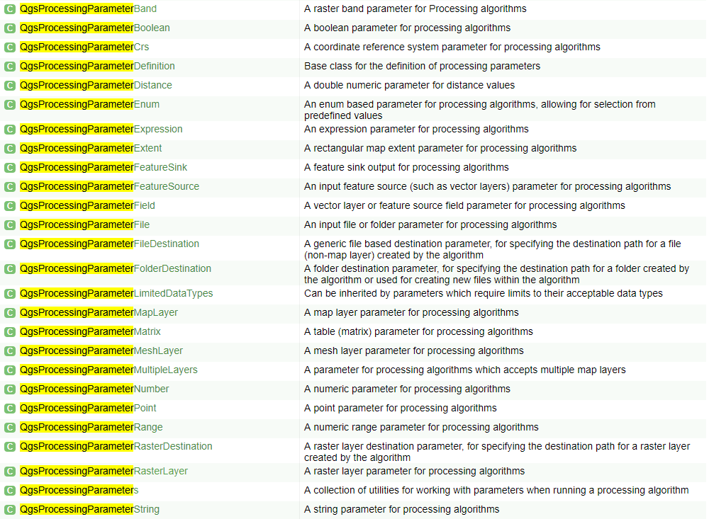
Tip
Get yourself familiarized with the full list of QGIS processing parameters. In the QGIS API Class List, search [Ctrl+F] for the term QgsProcessingParameter to find the list of available parameters.

Warning
The QGIS API Documentation is written in C++ terminology. At first, users who don’t know about C++ find it hard to understand C++ API Docs. However, over time it’s getting easier. Getting used to C++ terminology is inevitable.
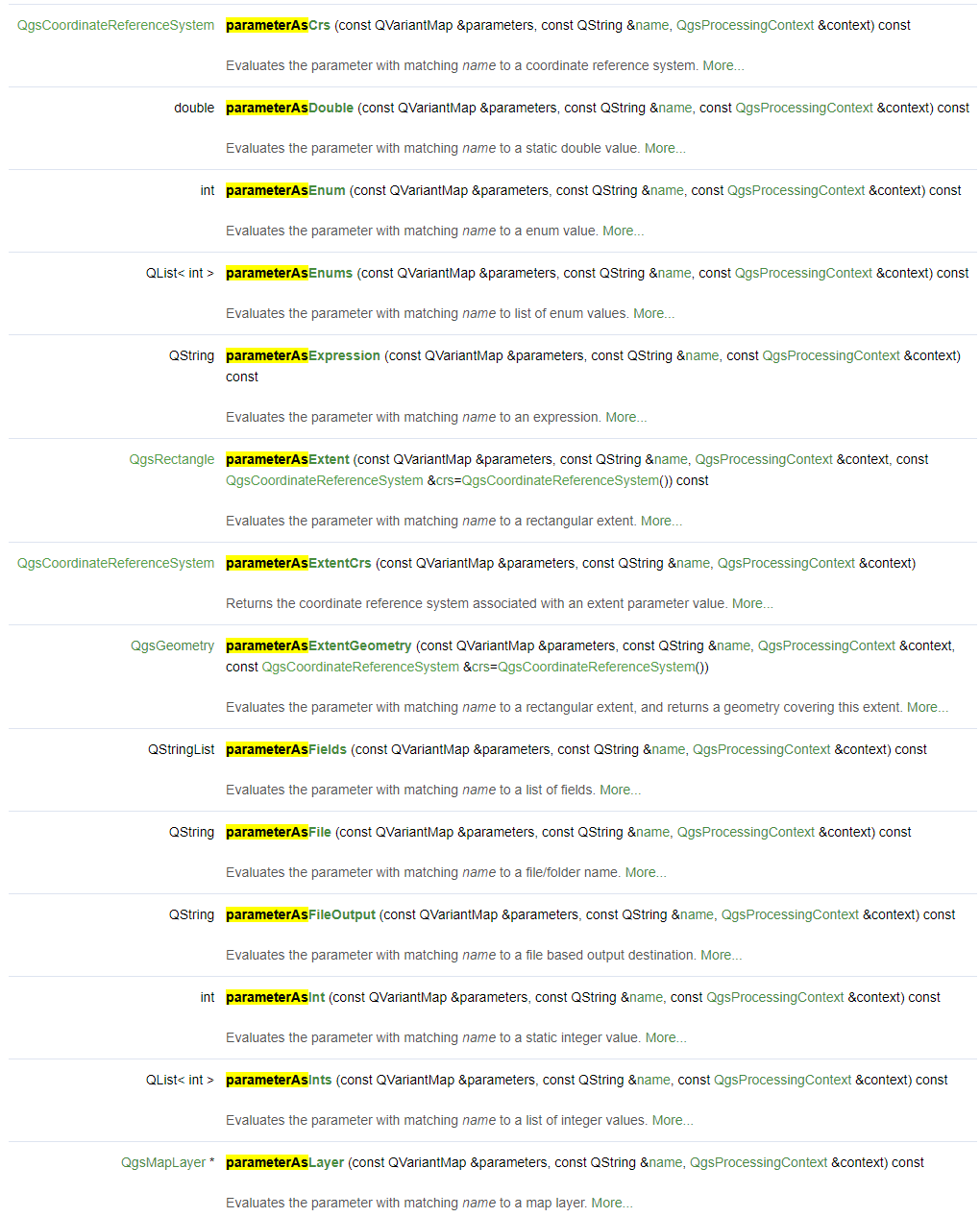
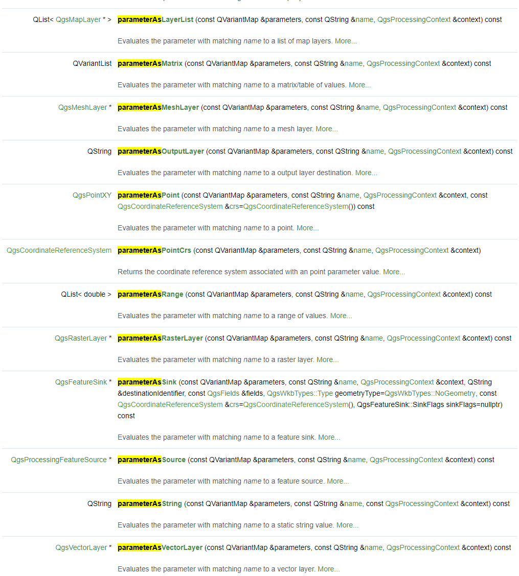
Define the processAlgorithm method that wraps the core algorithm implemented above.
With the various self.parameterAs<type>(parameters, self.P_<key>, context) evaluation statements, we query the selected user inputs and pass it to the core algorithm.
Finally, we return a dictionary of all created outputs.
Also note try-except idiom, that is used to handle any uncatched exceptions.
    def processAlgorithm(self, parameters, context, feedback):
        assert isinstance(feedback, QgsProcessingFeedback)

        # try to execute the core algorithm
        try:

            # pass all selected input parameters to the core algorithm
            regressionBasedUnmixing(
                filename=self.parameterAsOutputLayer(parameters, self.P_OUTPUT_FRACTION, context),
                rasterFilename=self.parameterAsRasterLayer(parameters, self.P_RASTER, context).source(),
                vectorFilename=self.parameterAsVectorLayer(parameters, self.P_VECTOR, context).source(),
                classAttribute=self.parameterAsString(parameters, self.P_FIELD, context),
                oversampling=self.parameterAsInt(parameters, self.P_OVERSAMPLING, context),
                coverage=self.parameterAsDouble(parameters, self.P_COVERAGE, context))

            # return all output parameters
            return {self.P_OUTPUT_FRACTION: self.parameterAsOutputLayer(parameters, self.P_OUTPUT_FRACTION, context)}

        # handle any uncatched exceptions
        except:
            # print traceback to console and pass it to the processing feedback object
            import traceback
            traceback.print_exc()
            for line in traceback.format_exc().split('\n'):
                feedback.reportError(line)
            return {}
Tip
Get yourself familiarized with the full list of evaluation methods. In the QgsProcessingAlgorithm documentation, search [Ctrl+F] for the term parameterAs to find the list of available evaluation methods.
Tip
Get yourself familiarized with the QgsProcessingFeedback class, which exposes various methods for providing progress feedback from the algorithm to the GUI.
Define a meaningful algorithm description which will be visible in the auto-generated GUI.
    def shortHelpString(self):

        html = '' \
       '<p>This algorithm derives landcover pixel fractions from the given raster and vector maps, fits a ' \
       '<a href="https://scikit-learn.org/stable/modules/generated/sklearn.ensemble.RandomForestRegressor.html">RandomForestRegressor</a> ' \
       'to that dataset and applies it to the the raster, predicting a (multi-class) landcover fraction map.</p>' \
       '<h3>Raster</h3>' \
       '<p>Input raster.</p>' \
       '<h3>Vector</h3>' \
       '<p>Input vector with landcover polygons.</p>' \
       '<h3>Class attribute</h3>' \
       '<p>Attribute defining the class ids (values between 1 and number of classes).</p>' \
       '<h3>Minimam pixel coverage</h3>' \
       '<p>Threshold between 0 and 1 that defines the minimal coverage a pixel must have to be concidered as training sample.</p>' \
       '<h3>Output fraction</h3>' \
       '<p>Output raster.</p>'
        return html
Provide a link to an external website, that is opened in the users web browser, when the Help button in the auto-generated GUI is clicked.
    def helpUrl(self, *args, **kwargs):
        return 'https://enmap-box.readthedocs.io/'
Define how a new instance of this class is created. Usually, this won’t change, unless you need to parametrize your algorithm at creation time (rare!).
    def createInstance(self):
        return type(self)()
This concludes the code discussion.
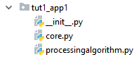
EnMAP-Box integration
To integrate the processing algorithm into the EnMAP-Box, create a folder structure with the above implemented core.py and processingalgorithm.py files:
In __init__.py we have to derive from the EnMAPBoxApplication class and implement a enmapboxApplicationFactory method which returns an instance of our application.
Here is a full listing of the implementation:
Code listing
from enmapbox.gui.applications import EnMAPBoxApplication
from tut1_app1.processingalgorithm import RegressionBasedUnmixingProcessingAlgorithm

def enmapboxApplicationFactory(enmapBox):
    return [RegressionBasedUnmixingApp(enmapBox)]

class RegressionBasedUnmixingApp(EnMAPBoxApplication):
    def __init__(self, enmapBox, parent=None):
        super().__init__(enmapBox, parent=parent)

        self.name = 'Regression-based Unmixing Application'
        self.version = 'dev'
        self.licence = 'GNU GPL-3'

    def processingAlgorithms(self):
        return [RegressionBasedUnmixingProcessingAlgorithm()]
Test environment
Here is a test setup using the EnMAP-Box testdata:
from enmapbox.gui.enmapboxgui import EnMAPBox
from enmapbox.testing import initQgisApplication
from tut1_app1 import RegressionBasedUnmixingApp

if __name__ == '__main__':

    qgsApp = initQgisApplication()
    enmapBox = EnMAPBox(None)
    enmapBox.run()
    enmapBox.openExampleData(mapWindows=1)
    enmapBox.addApplication(RegressionBasedUnmixingApp(enmapBox=enmapBox))
    qgsApp.exec_()
    qgsApp.exitQgis()
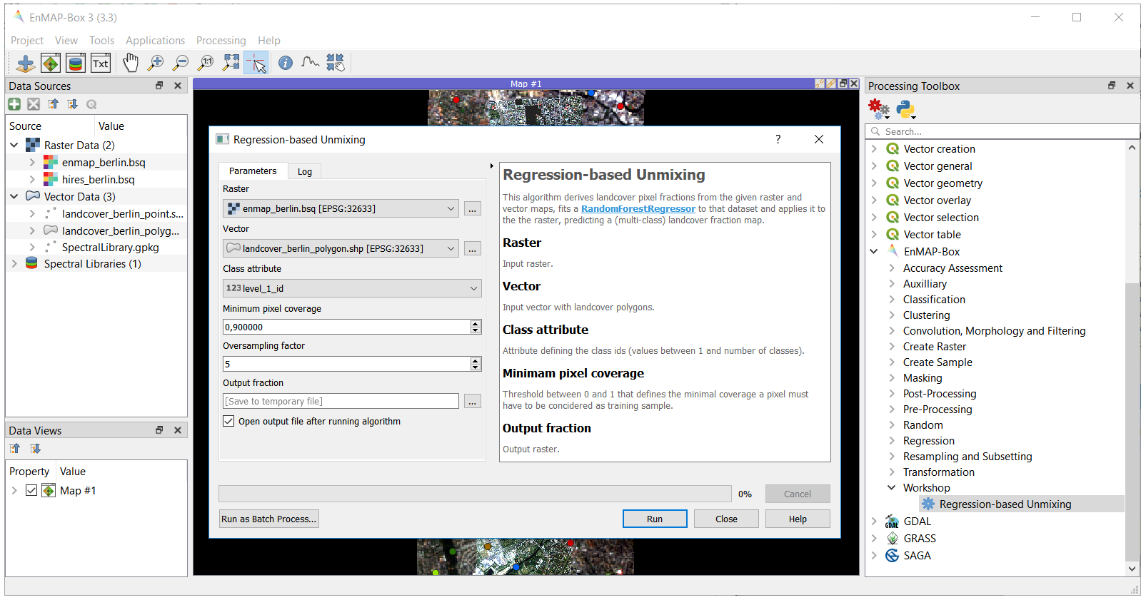
Task
Open and run the test_app.py script in PyCharm.
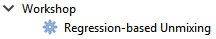
After the EnMAP-Box is loaded, navigate to EnMAP-Box > Workshop > Regression-based Unmixing in the Processing Toolbox panel and execute the algorithm..
Deployment
Up to now, the application is only visible after adding it programmatically to the EnMAP-Box via:
enmapBox.addApplication(RegressionBasedUnmixingApp(enmapBox=enmapBox))
To also show it in the EnMAP-Box opened inside QGIS, we have two options:
Insert the application folder path into the /enmapbox/coreapps/enmapboxapplications.txt file:
# this file describes other locations of EnMAP-Box applications
# just give the PATH relative to the root directory

C:\source\enmap-box-workshop2019\programming_tutorial1\tut1_app1
or
Copy the application folder into the /enmapbox/apps folder:
/enmapbox
    /apps
        /tut1_app1
Note
If you want your application shipped together with the EnMAP-Box, contact us:
Andreas Rabe (andreas.rabe@geo.hu-berlin.de)