Regression-based mapping of forest aboveground biomass

Authors: Sam Cooper, Akpona Okujeni, Patrick Hostert, Clemens Jaenicke, Benjamin Jakimow, Andreas Rabe, Fabian Thiel & Sebastian van der Linden

Publication date: 03/07/2020

Last update: 02/08/2022

Introduction

1. Background

This tutorial is part of the HYPERedu online learning platform, an education initiative within the EnMAP mission hosted on EO College. HYPERedu provides annotated slide collections and hands-on tutorials using the open-source EnMAP-Box software, targeting basic principles, methods as well as applications of imaging spectroscopy.

Annotated slide collections for the tutorial Regression-based mapping of forest aboveground biomass and a software description unit for the EnMAP-Box are provided here:

• Slide collection
• Software description

2. Content

Forest aboveground biomass (AGB) is a measure of the living and dead plant material in a given area. As such, it is often used for forest management, assessing fire potential, and is an important metric used in modelling carbon and nutrient cycles. AGB can be directly measured at a plot level by harvesting and weighing vegetation, but this is both an expensive and highly invasive process. Through the use of statistical modelling and remotely sensed imagery, AGB can be mapped across broad, spatially continuous areas using only a small number of directly measured reference plots. This tutorial focuses on regression-based modeling of forest AGB using the EnMAP-Box. A hyperspectral image mosaic from the EnMAP sensor (here simulated from AVIRIS imagery) and a corresponding vector dataset containing plot-based AGB references are used for this tutorial. The aim is to provide an introduction into the functionality of the EnMAP-Box, as well as hands-on training for implementing regression-based mapping.

3. Requirements

This tutorial requires at least version 3.10 of the EnMAP-Box 3. There might be some minor changes for higher versions (e.g., changed menu labels, added parameter options, etc.).

4. Further reading

We recommend [1] and [2] for a comprehensive overview of imaging spectroscopy of terrestrial ecosystems, [3] for an overview of remote sensing of forest AGB and [4] for a companion study using the same data.

[1]	Foerster, S., Guanter, L., Lopez, T., Moreno, J., Rast, M., Schaepman, M.E. (2019) Exploring the Earth System with Imaging Spectroscopy. Springer International Publishing

[2]	Thenkabail, P. S., & Lyon, J. G. (2016). Hyperspectral remote sensing of vegetation. CRC press.

[3]	Lu, D., Chen, Q., Wang, G., Liu, L., Li, G., & Moran, E. (2016). A survey of remote sensing-based aboveground biomass estimation methods in forest ecosystems. International Journal of Digital Earth, 9(1), 63-105.

[4]	Cooper, S., Okujeni, A., Pflugmacher, D., van der Linden, S., & Hostert, P. (2021). Combining simulated hyperspectral EnMAP and Landsat time series for forest aboveground biomass mapping. International Journal of Applied Earth Observation and Geoinformation, 98.

5. Data

You can download the data for this exercise here:

https://box.hu-berlin.de/f/d73fa3ba95c143388832/?dl=1

The tutorial data contains a simulated hyperspectral EnMAP image, plot-based AGB references as well as a land cover map for a small study area located in Sonoma County, California, USA. The simulated EnMAP image is a subset extracted from the “2013 Simulated EnMAP Mosaics for the San Francisco Bay Area, USA” dataset [5]. AGB reference data was sampled from an existing LiDAR derived AGB map [6]. The land cover map was taken from the 2011 National Landcover Database (NLCD) [7].

Data type	Filename	Description
Raster	enmap_sonoma.bsq	Simulated spaceborne hyperspectral data from the EnMAP sensor with a spatial resolution of 30m, 195 bands, and 1000x200 pixels (ENVI Standard Band Sequential bsq)
Raster	nlcd_sonoma.bsq	National Land Cover Database 30m classification for the study region (ENVI Standard Band Sequential bsq)
Vector	agb_sonoma.gpkg	343 AGB reference points sampled from the existing LiDAR derived AGB map (GeoPackage gpkg)

[5]	Dubayah, R.O., A. Swatantran, W. Huang, L. Duncanson, H. Tang, K. Johnson, J.O. Dunne, and G.C. Hurtt. 2017. CMS: LiDAR-derived Biomass, Canopy Height and Cover, Sonoma County, California, 2013. ORNL DAAC, Oak Ridge, Tennessee, USA. https://doi.org/10.3334/ORNLDAAC/1523

[6]	Cooper, S.; Okujeni, A.; Jänicke, C.; Segl, K.; van der Linden, S.; Hostert, P. (2020): 2013 Simulated EnMAP Mosaics for the San Francisco Bay Area, USA. GFZ Data Services. https://doi.org/10.5880/enmap.2020.002

[7]	Multi-Resolution Land Characteristics Consortium (MRLC) (2018). National Land Cover Database 2011 (NLCD 2011). Multi-Resolution Land Characteristics Consortium (MRLC). https://data.nal.usda.gov/dataset/national-land-cover-database-2011-nlcd-2011. Accessed 2022-08-08.

Exercise A: Getting started with the EnMAP-Box

Description

This exercise introduces basic functionalities of the EnMAP-Box for this tutorial. You will get to know the graphical user interface and will learn how to load data, visualize raster and vector data, and use the basic navigation tools. Additionally, you will learn to work with multiple map views and how to visualize image spectra using Spectral Library Windows.

Duration: 30 min

1. Start the EnMAP-Box

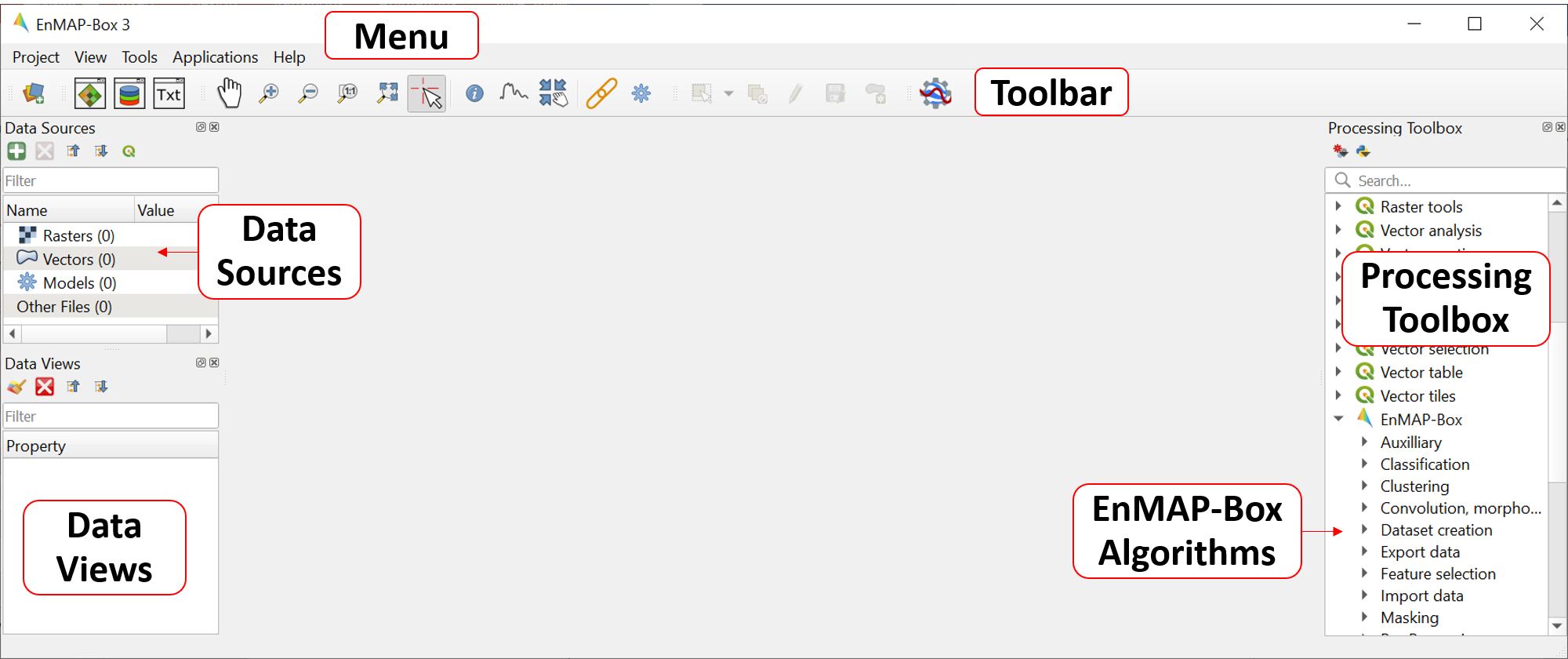
• Start QGIS and click the icon in the toolbar to open the EnMAP-Box. The GUI of the EnMAP-Box consists of a Menu and a Toolbar as well as panels for Data Sources and Data Views.
• The QGIS Processing Toolbox including the EnMAP-Box algorithms can be optionally added to the GUI by clicking on View in the Menu and by checking the Processing Toolbox from the Panel list.

2. Load data

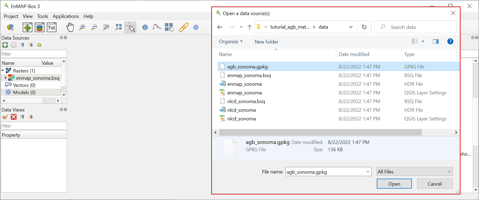
• To load new datasets into the EnMAP-Box, click the icon and navigate to the file directory containing your data. Select agb_sonoma.gpkg from the Open data source dialogue and select Open.
• Alternatively, the EnMAP-Box offers simple drag & drop capabilities to load data from an external file manager (e.g. Windows File Explorer). Load enmap_sonoma.bsq by dragging and dropping the file from your file manager into the Data Sources panel.
• All data currently open in the EnMAP-Box will appear in the Data Sources panel.

3. Visualize raster data

• The EnMAP-Box offers Map Views (Map #) for visualizing raster and vector data. Click the icon to open a new Map View and drag enmap_sonoma.bsq from the Data Sources panel into Map #1.

• In addition to a new Map View opening, a corresponding Data View entry is created in the Data Views panel which shows all data currently loaded in a given Map View.

• The enmap_sonoma.bsq image will be displayed as true color RGB composite. True color rendering is based on predefined RGB band combinations (R: 658 nm, G: 569 nm, B: 479 nm) stored in the QGIS Style File enmap_sonoma.qml.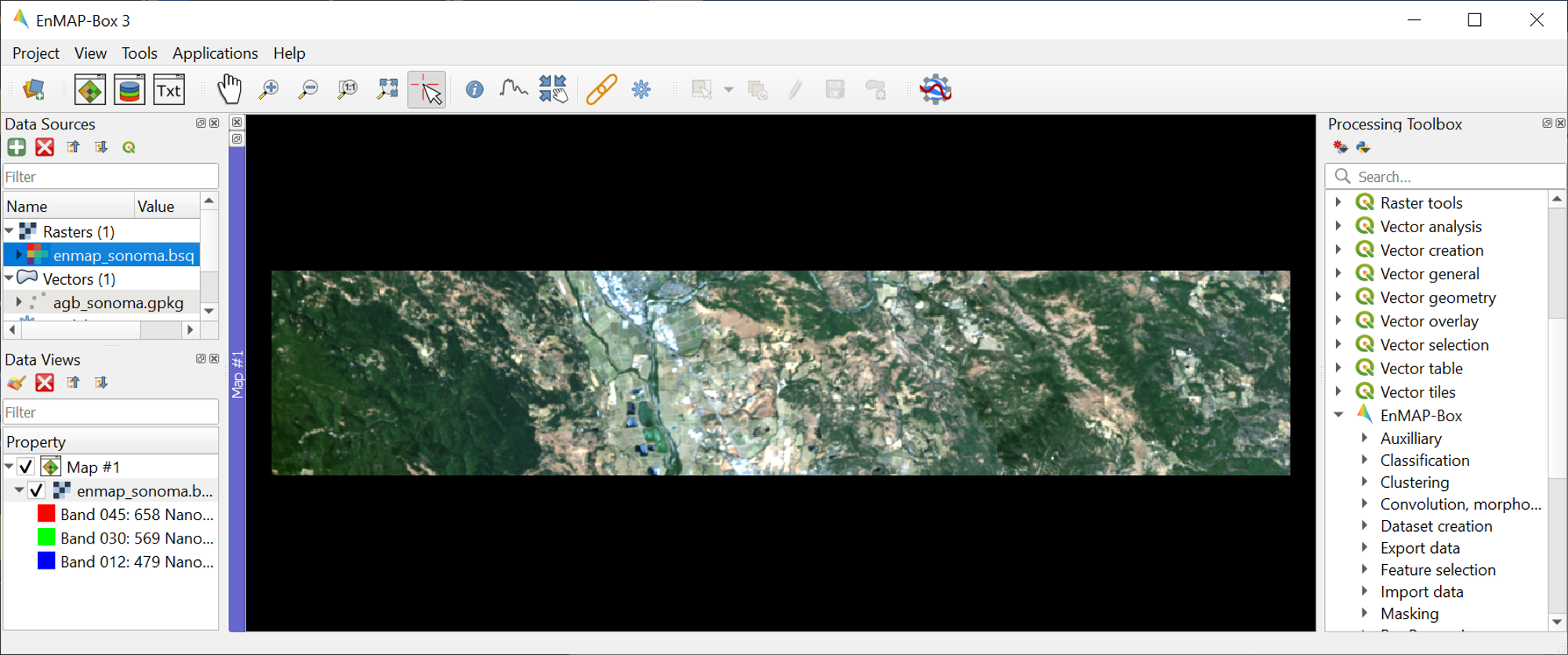

  

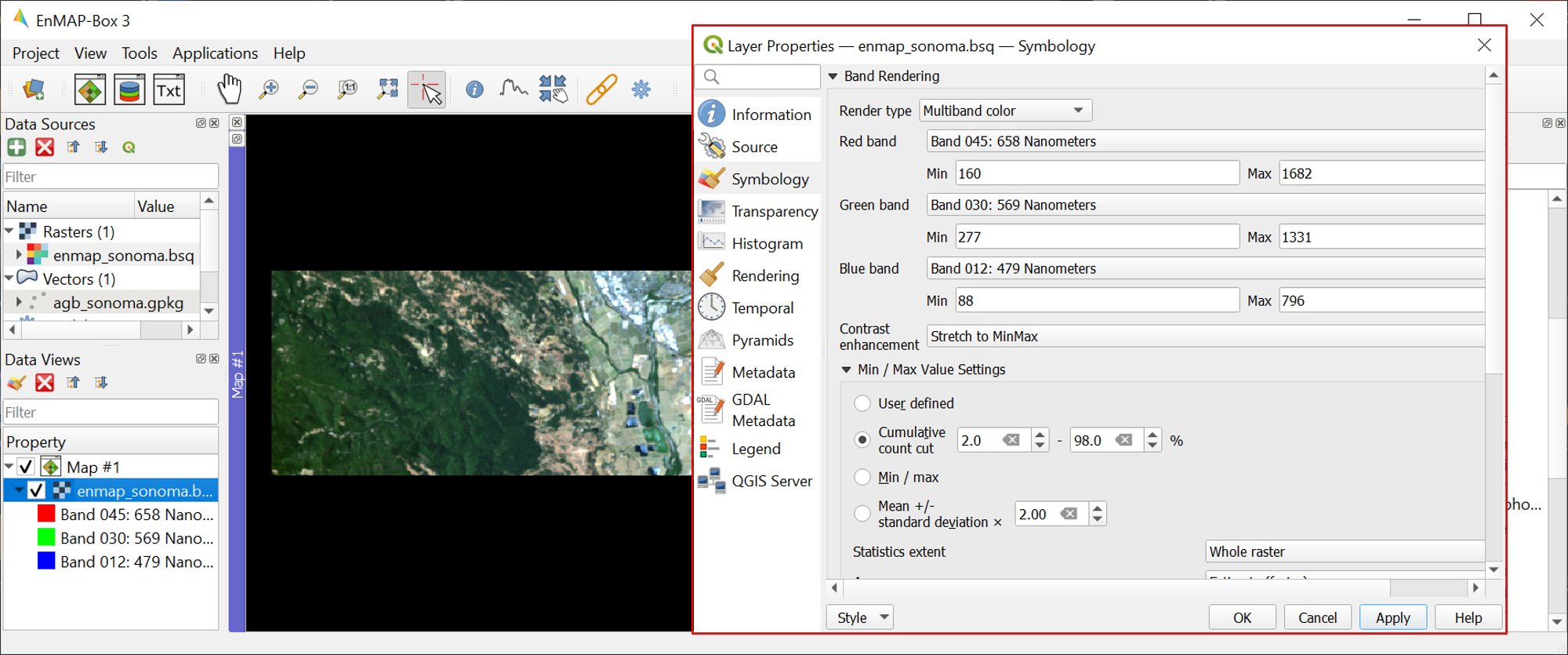
• To assign a different RGB combination to the RGB channels, right click on the dataset in the Data Views panel, select

Layer Properties and navigate to Symbology. Set Render type to Multiband color and select bands to display in the red, green and blue color channels. Choose appropriate Min/Max Value Settings (e.g. Cumulative Count Cut: 2-98%). Common RGB combinations are listed below.

Combination	Red	Green	Blue
TrueColor	658 nm	569 nm	479 nm
nIR	847 nm	658 nm	569 nm
swIR	847 nm	1645 nm	658 nm

Tip

If the raster image has wavelength information associated with it, you may also select an RGB combination from different custom RGB band combinations (True Color, Colored IR, SWIR-NIR-R or NIR-SWIR-R). Right click on the dataset in the Data Views panel, select Layer Properties and navigate to Raster Band. Don’t forget to choose appropriate Min/Max Value Settings.

4. Basic navigation tools

• The Toolbar offers common navigation tools for exploring visualized datasets. Make yourself familiar with the following navigation tools:
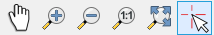
• Note that the mouse wheel can be used alternatively for zooming (roll mouse wheel forward/backward) and panning (press and hold mouse wheel).
• For a better orientation when exploring visualized raster images, you may switch on the crosshairs (right click into Map View and activate Crosshair ‣ Show.
• Make yourself familiar with the icon on the toolbar to view pixel values of the displayed raster. Note: ^{Identify Cursor Info} must be activated to access this tool. When activated and used, a new Cursor Location Values window will open displaying data from the selected pixel. This tool similarly works for viewing attribute information of displayed vector data.

5. Multiple map views

• The EnMAP-Box enables users to work with multiple Map Views, which can be flexibly organized and geospatially linked.

• Open a new Map View (Map #2) by clicking the icon.

  Note

  A new Data view appears corresponding to the newly added Map View.

• Display enmap_sonoma.bsq as an RGB composite of your choice in Map #2.

Tip

When loading a raster image to a map view, you may also right click the filename in the Data Sources panel and select either Open in existing map or Open in new map. If the raster image has wavelength information associated with it, you may also select a predefined composite from the context menu.

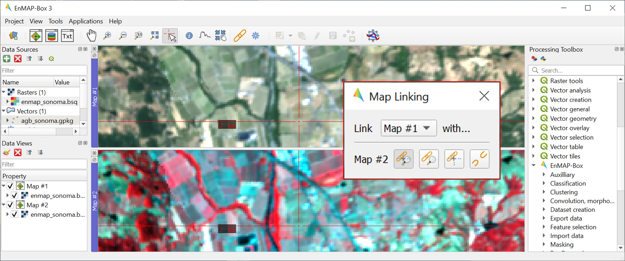
• For geospatial linking, click on View in the Menu and select Set Map Linking. In the Map Linking window, select the Link Map Scale and Center option and close the dialog. You may also right click a map window and select Link with other maps to initialize the linking process.

Tip

Map Windows can be re-arranged by clicking on the blue Map title bar (Map #) and dragging it to the desired position. A transparent blue rectangle will appear indicating the docking position once you release the mouse button. You may also undock map views from the EnMAP-Box window by selecting from the blue Map title bar. To re-dock a Map View, click and drag the blue Map title bar to an open Map View already docked in the EnMAP-Box window.

6. Visualize vector data

• Close Map #2 from the previous step.

• Load agb_sonoma.gpkg to Map #1.

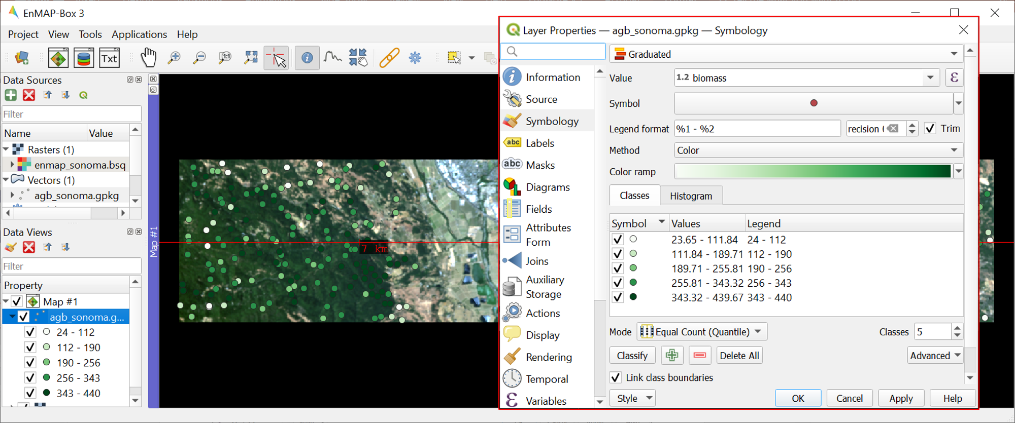
• To change the order of stacked layers, go to the Data Views panel and drag one layer on top or below another one. Arrange the layer stack so that agb_sonoma.gpkg is displayed on top of enmap_sonoma.bsq.

• By default, vector files are displayed with a single uniform symbol. To change this symbology, right click on agb_sonoma.gpkg in the Data Views panel, select Layer Properties and navigate to Symbology in the Layer Properties window. You can now change the symbology in accordance to the QGIS functionality.

  • Select Graduated from the dropdown menu, and select biomass in Value and Color in Method.
  • Set the Color ramp to run from white to green.
  • Press Classify and then OK to display the biomass values associated with each point.

7. Extract & visualize image spectra

• The EnMAP-Box offers Spectral Library Windows (SpectralLibrary #) for visualizing spectra and handling their metadata.

• This tool may also be used to extract and visualize spectra which are spatially associated with vector data open in the EnMAP-Box, i.e., the AGB reference points. To do this, open a new Spectral Library window by selecting the icon on the toolbar.

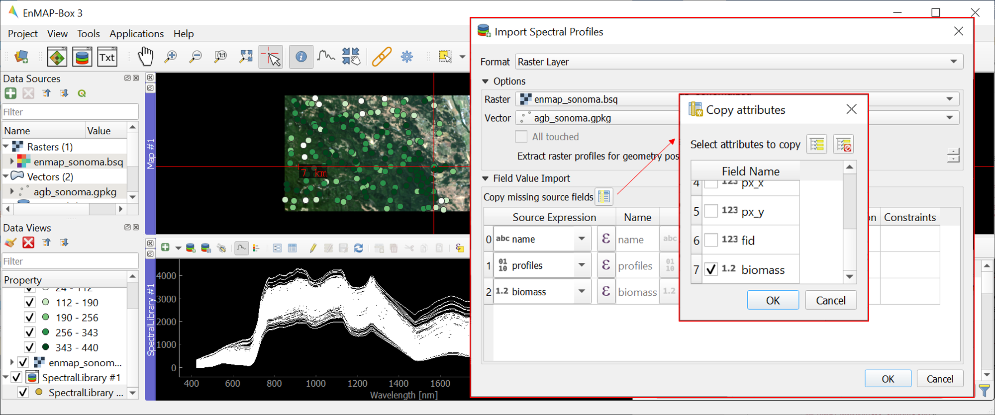
• Next, import spectral profiles from other sources by clicking at the icon in the SpectralLibrary #1 menu. Specify the following settings:

  • Format = Raster Layer
  • Options: Raster = enmap_sonoma.bsq, Vector = agb_sonoma.gpkg
  • Field Value Import: Click on the icon, select biomass and click OK.

• Terminate the Import Spectral Profile dialogue with OK. A spectral library is automatically built based on the geographic location of each point in the vector file. The associated attribute information is displayed in the table on the right.

• In Exercise B, you will learn how to create regression models based on the illustrated spectra and related AGB quantities to predict AGB across the whole image.

Learning Activities

• A1: What land cover types are present in the imagery? How are the AGB reference plots distributed throughout the scene?
• A2: What different information can you see when switching from a true color composite to a NIR false color composite?

Exercise B: Regression based mapping of AGB

Description

One of the strengths of remote sensing comes from its ability to take high-quality plot measurements of a variable of interest and building statistical models with which wall to wall maps of this variable can be created. One of the most common ways of doing this is to create regression models based on the optical properties of the training data and applying it to large scale imagery. This exercise …

• Introduces a regression-based mapping approach for taking plot measurements of AGB and generating spatial AGB estimates using an input raster of hyperspectral imagery.
• Demonstrates the Regression Dataset Manager and the Regression Workflow applications of the EnMAP-Box.

Duration: 20 min

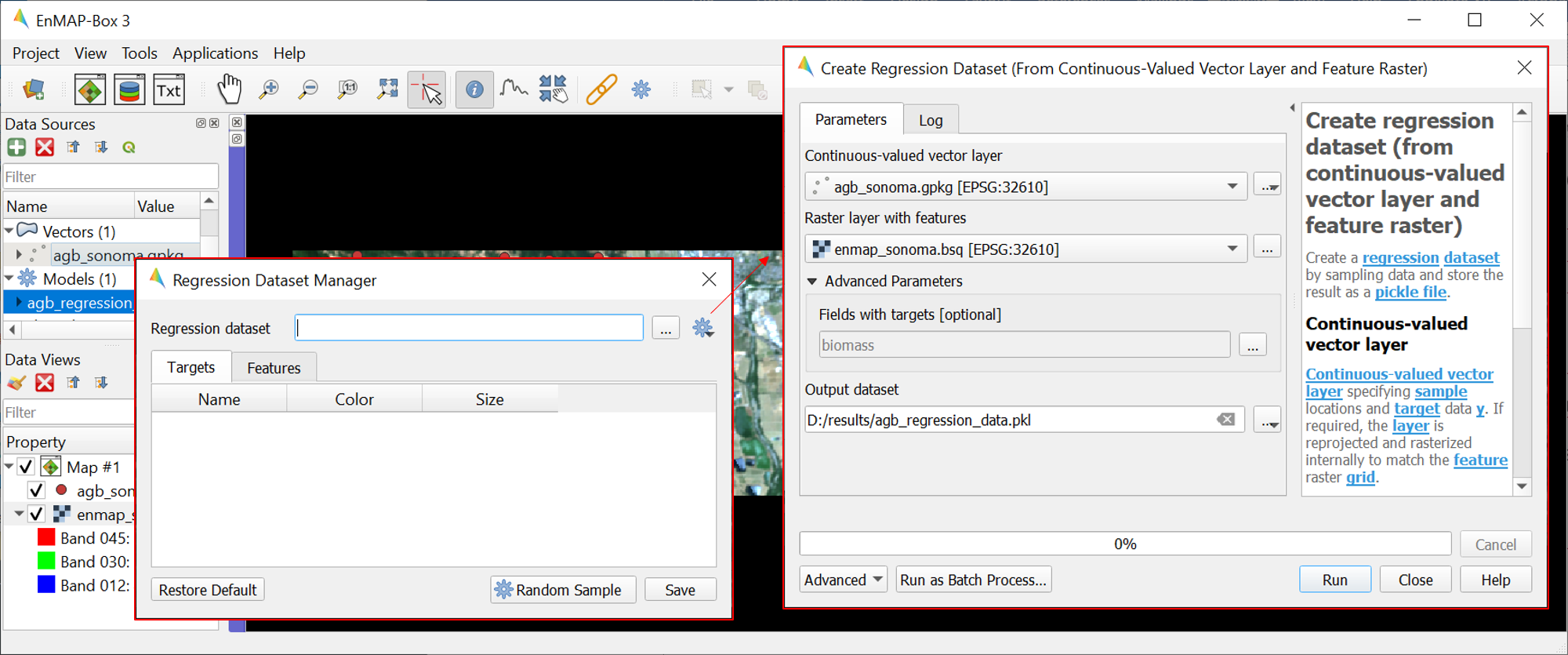
1. Use the Regression Dataset Manager for data preparation

• The Regression Dataset Manager offers different options to prepare data for the Regression Workflow application. In the context of this tutorial, you will create a Regression Dataset from a raster and a vector layer containing the spectral features (independent variable) and the target variable (dependent variable), respectively. The regression dataset will be stored as pickle file (.pkl).

• Open enmap_sonoma.bsq and agb_sonoma.gpkg in a single Map Window. Close all other opened Map and Spectral Library Windows.

• Click on Applications in the Menu and select Regression Dataset Manager.

• To create the Regression Dataset from a raster and a vector layer, click on the icon and choose Create regression dataset (from continuous-valued vector layer and feature raster). A new widget will be opened. Run the dialog with the following inputs:

  • Continuous-valued vector layer: select agb_sonoma.gpkg
  • Raster layer with features: select enmap_sonoma.bsq
  • Fields with targets: select attribute biomass
  • Output Data: select … ‣ Save to File… and define an output path and file name (e.g. agb_regression_data.pkl).

• After running the dialog, agb_regression_data.pkl will be opened under Models in the Data Sources panel. Close the Regression Dataset Manager.

Tip

The Regression Dataset Manager offers different random sampling options, e.g. for splitting Regression data into training and validation data. Once the Regression data is prepared, you can access these options through the Random Sample button.

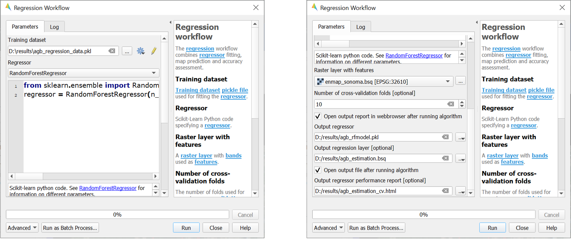
2. Use the Regression Workflow for estimating AGB

• The Regression Workflow application offers several state-of-the-art regression algorithms from the scikit-learn library (see https://scikit-learn.org/stable/index.html) for predicting continuous variables. The application further includes an optional cross-validation for assessing model performances.

• Click on Applications in the Menu and select Regression Workflow to open the regression application.

  • Choose agb_regression_data.pkl as Training dataset.
  • Select RandomForestRegressor (default, due to the low processing time) as Regressor, and use the default model parameters. Note that the different algorithms provided lead to varying accuracies and processing times. Refer to the scikit-learn documentation for more information.
  • Raster layer with features specifies the raster image to which the regression model will be applied. Select enmap_sonoma.bsq. Specify output path and file name (e.g. agb_estimation.bsq) under Output regressor layer to save the result in your working directory.
  • To make use of a cross-validation, set the Number of cross-validation folds to 10 (default) and leave the Open output performance report option checked. Specify output path and file name (e.g. agb_estimation_cv.html) under Output regressor performance report to save the report in your working directory.
  • The regression model can be optionally saved, e.g. for applying the model again to a dataset. Specify output path and file name (e.g. agb_rfmodel.pkl) under Output regressor to save the result in your working directory.
  • Click run to start the Regression Workflow.

Tip

All processing options of the Regression Workflow that are labeled as [optional] can be disregarded by setting the Output to Skip Output.

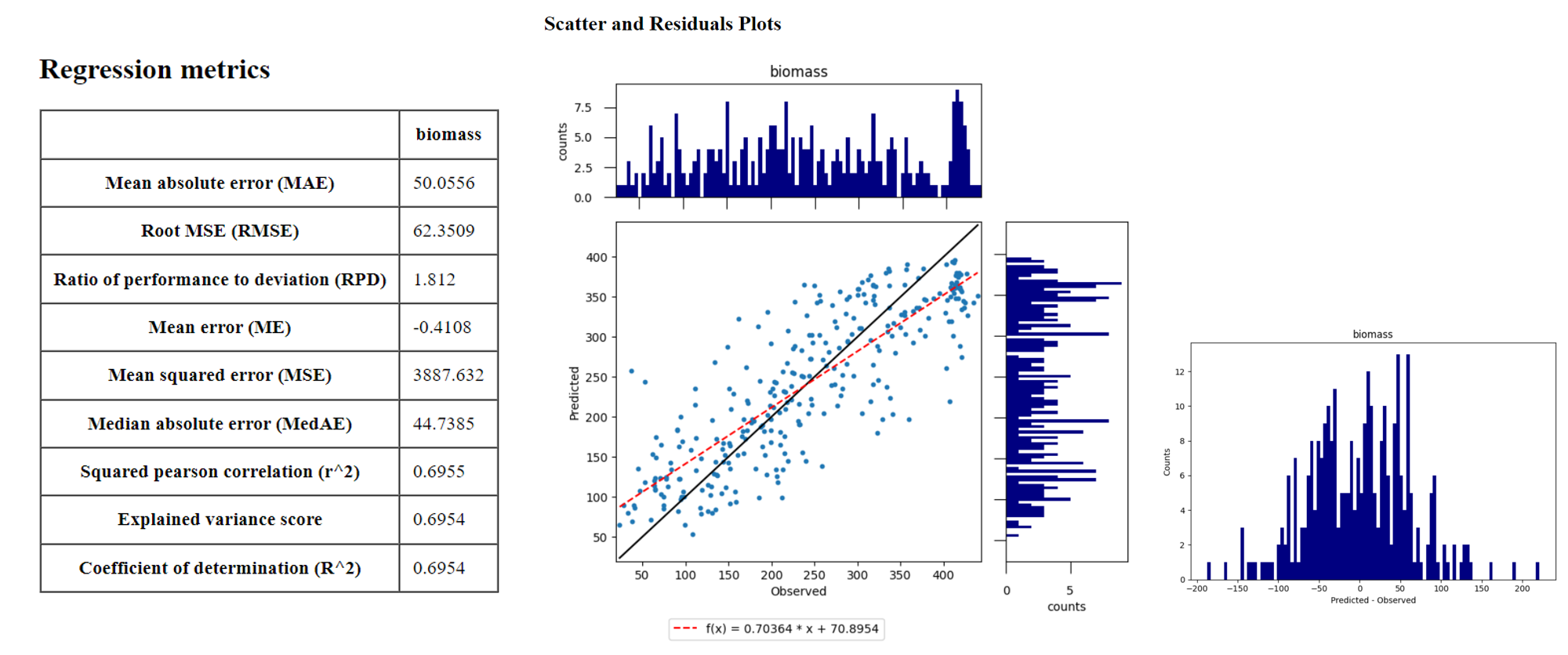
3. Assess the model performance for AGB estimation

• After running the Regression Workflow, the performance report with scatterplots and statistical measures will be opened in your default web browser.
• Based on the 10-fold cross-validation, you can now access the performance of your model to predict AGB.

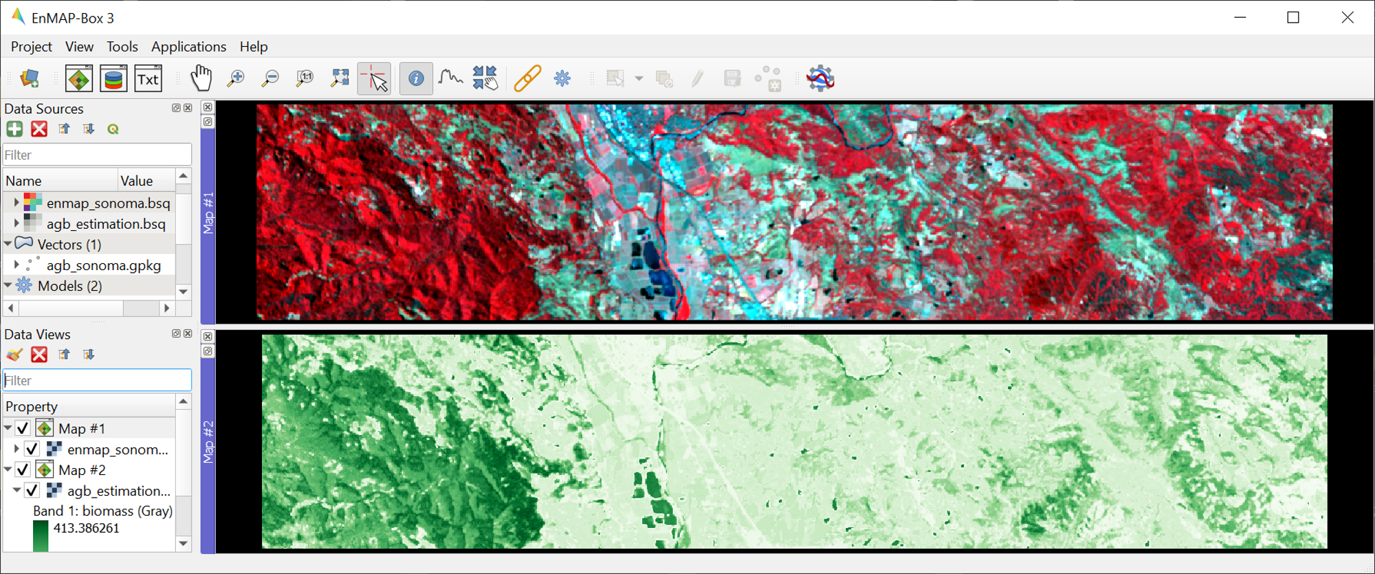
4. Visualize AGB results

• After running the Regression Workflow, all outputs will appear in the Data Sources panel.
• Close all opened Map/SpectralLibrary Windows. Open enmap_sonoma.bsq as an RGB composite of your choice in Map #1.
• Open the agb_estimation.bsq in a new Map View and link to the Map #1. Use the Layer Properties to change the color ramp to white-green (Singleband pseudocolor).

Learning Activities

Learning Activities

• B1: What general trends do you see in the biomass estimations? How do they compare to landscape features seen in the EnMAP imagery?
• B2: Discuss the accuracy results, both in terms of the statistical measures, as well as the form of the scatterplot and histograms.

Exercise C: Compare AGB estimates with the NDVI

Description

In this exercise, you will learn how to use the ImageMath application to calculate a NDVI map and generate a forest mask based on the NLCD land cover map. Based on the forest area only, you will then assess the AGB prediction from Exercise B relative to the NDVI using the Scatter Plot Tool.

Duration: 30 min

1. Introduction to ImageMath

• The ImageMath tool in the EnMAP-Box allows users to apply a mathematical operation, python function or user defined function to an image. In the following sections, you will utilize standard numpy array processing protocols

  • to calculate a NDVI map from two bands of our EnMAP imagery,
  • to generate a forest mask from the NLCD land cover map,
  • and to apply a forest mask to both the NDVI and AGB maps.

• Close all opened Map/Spectral Library Windows. Display enmap_sonoma.bsq, nlcd_sonoma.bsq and agb_estimation.bsq in a single or in multiple Map Views.

• Open the ImageMath application by going to Applications then selecting ImageMath

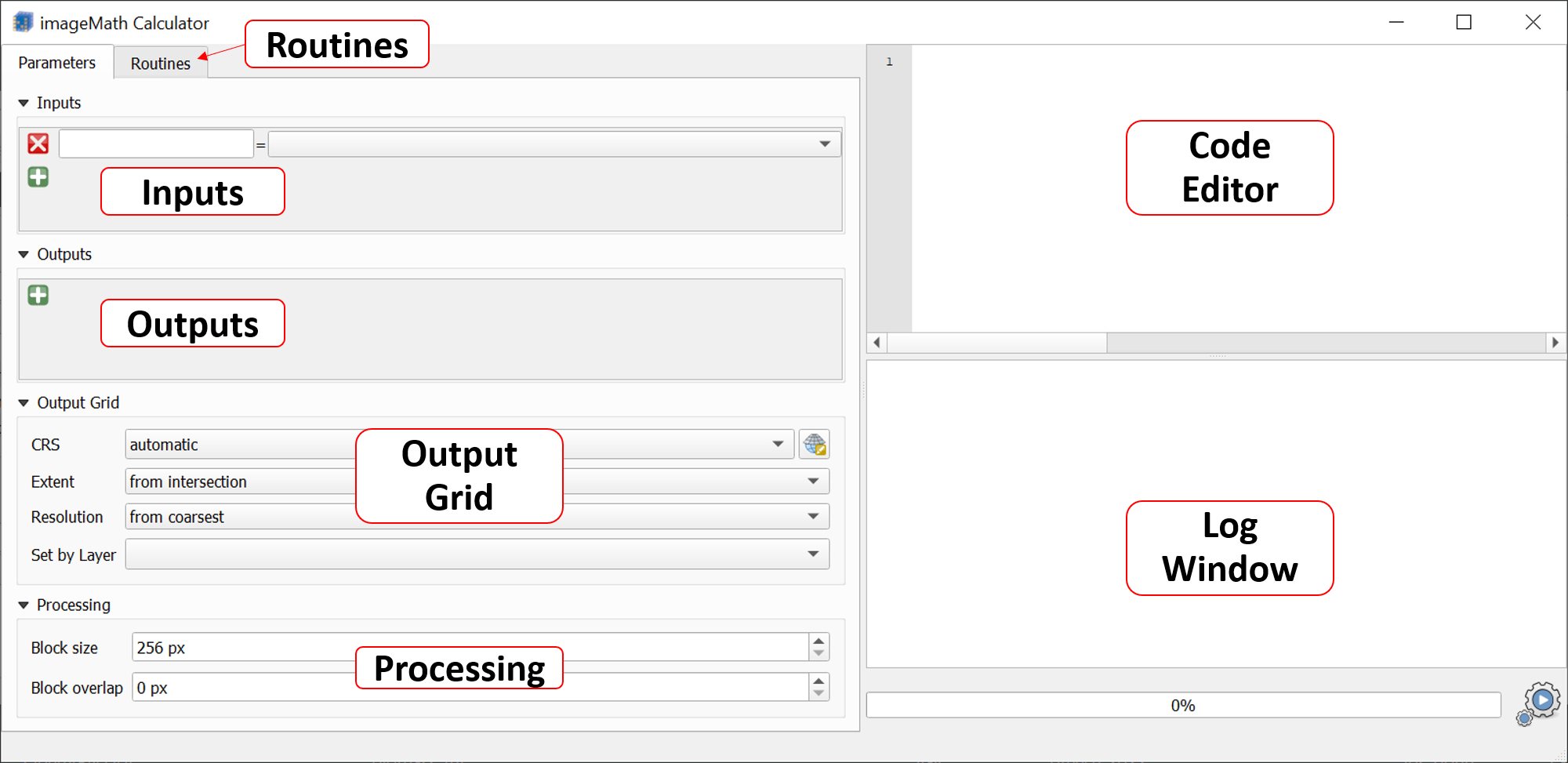
• ImageMath consists of several panels:

  • Inputs: defines input variables and variable names.
  • Outputs: defines output variable names and locations to be saved to.
  • Code editor: Text editor in which programmatic manipulation of the input datasets can be defined using Python scripting syntax.
  • Output Grid: Allows users to manually set the output grid.
  • Processing: Allows users to select block sizes for processing large datasets with limited memory.
  • Log Window: Displays the status (and error messages) of executed code.
  • Additionally, a tab for Routines allows users to select a number of common python-based tools for manipulating spatial datasets with linked documentation.

2. Calculate NDVI

• The Normalized Difference Vegetation Index (NDVI) is a commonly used vegetation index that is correlated with both vegetation cover and AGB. The formula for NDVI is:

  \[NDVI = \frac{NIR-Red}{NIR+Red}\]

  where NIR is the near-infrared band reflectance (~850nm) and Red is the red band reflectance (~660nm). We will now calculate NDVI from the EnMAP imagery using ImageMath.

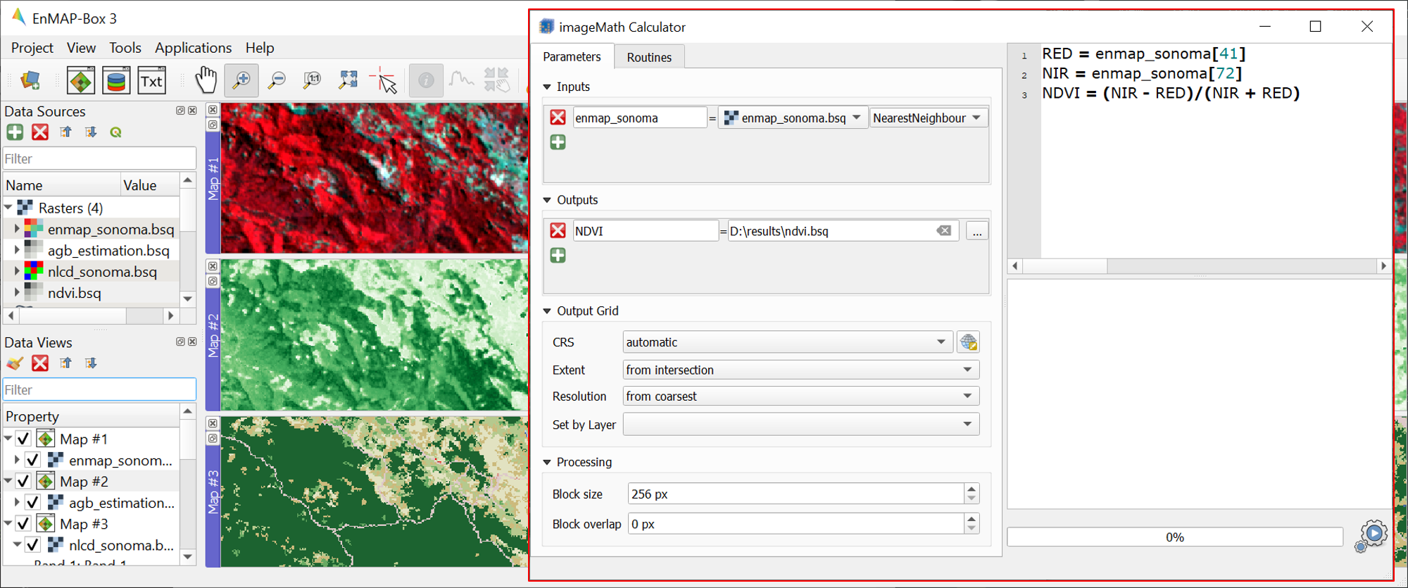
• In the Inputs panel, select enmap_sonoma.bsq from the dropdown menu. The variable name is automatically taken from the filename, but may be changed if desired.

• In the Code Editor, define the RED and NIR bands in our EnMAP imagery. These correspond to bands 42 and 73, respectively, and we can define them using python indexing syntax (i.e. 0 indexed array slicing):

  RED = enmap_sonoma[41]
  NIR = enmap_sonoma[72]
  

  Next, we define the formula we wish to run:

  NDVI = (NIR - RED)/(NIR + RED)
  

  In the Outputs panel, define the output variable name as NDVI, and select an output file path and file name (e.g. ndvi.bsq).

• Finally, click on the button to run the script. A new raster dataset ndvi.bsq will appear in the Data Sources panel.

Attention

Input and output variable names in the Code Editor must exactly match corresponding names defined in the Inputs and Outputs panels.

3. Create a forest mask

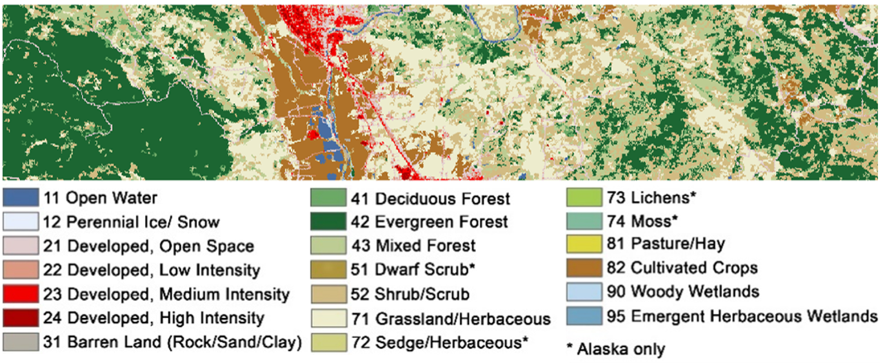
• As the model was trained using AGB reference plots from forest areas, only limited inference can be made of the non-forest AGB estimates. We will therefore apply a forest mask to our AGB map as well as to the NDVI map. The forest mask will be generated based on the available NLCD land cover map.
• Below are the NLCD classes and color legend represented in the raster data. We will consider any pixel to be forest which is labelled as Deciduous (41), Evergreen (42), or Mixed (43) forest according to the NLCD classification.

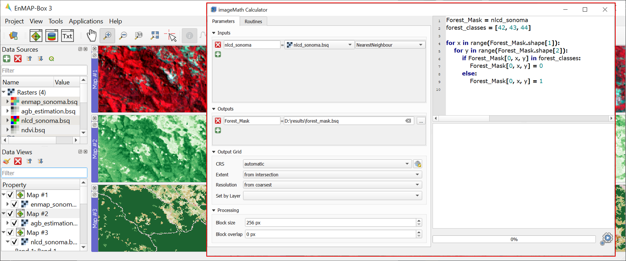
• Open the ImageMath application and set nlcd_sonoma.bsq as the input file.

• Enter the following code into the code editor:

  Forest_Mask = nlcd_sonoma
  forest_classes = [42, 43, 44]
  
  for x in range(Forest_Mask.shape[1]):
      for y in range(Forest_Mask.shape[2]):
          if Forest_Mask[0, x, y] in forest_classes:
              Forest_Mask[0, x, y] = 0
          else:
              Forest_Mask[0, x, y] = 1
  

• Line by line, this

  1. Copies the NLCD information to a new object we will manipulate to create the mask
  2. Creates a list of classes which we consider forest
  3. Loops through the x dimension of the raster. For each loop, x will be an integer representing the current location in the x dimension.
  4. Loops through the y dimension of the raster. For each loop, y will be an integer representing the current location in the y dimension. These two loops allow us to look at each element in the array individually. While numpy offers more efficient ways to analyse arrays (See section C4), this is one basic approach.
  5. Check if the element at the current x and y position is in the forest_classes list
  6. If it is, set that value to 0
  7. If it is not
  8. Set that value to 1

• Set Forest_Mask as the output and define the path and file name (e.g. forest_mask.bsq) for saving the result.

• Run the script by clicking .

• A new raster dataset forest_mask.bsq will appear in the Data Sources panel. The resulting mask now has a value of 0 for forested pixels, and 1 for non-forested pixels.

4. Apply the forest mask

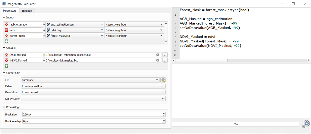
• Open the ImageMath application and set agb_estimation.bsq, ndvi.bsq and forest_mask.bsq as the input files. Note that these datasets need to be opened in a single or in multiple Map Views to make them selectable input files.
• Enter the following code into the Code Editor to apply the forest mask to the AGB and NDVI images.

Forest_Mask = forest_mask.astype(bool)

AGB_Masked = agb_estimation
AGB_Masked[Forest_Mask] = -99
setNoDataValue(AGB_Masked, -99)

NDVI_Masked = ndvi
NDVI_Masked[Forest_Mask] = -99
setNoDataValue(NDVI_Masked, -99)

• Line by line, this script:
  1. Sets the mask to a Boolean data type (i.e. True/False). The mask file contains binary values where 0 indicates forest (i.e. non-masked pixels) and 1 indicates non-forest (i.e. pixels to be ignored). In Python, 1 also represents True while 0 represents False, and by setting the datatype to bool, we explicitly tell Python to treat these values in this manner.
  2. Copies the AGB values to a new array.
  3. Steps through each value in the new array and sets the value to -99 if the mask value is True. In numpy array speak, this line can therefore read: “For each value in AGB_Masked, if the corresponding value in Forest_Mask is True (i.e. non-forest), then set that value to -99”. If the mask value is False (i.e. forested), nothing will happen, and the biomass value will remain in the array.
  4. Sets the no data value for the masked array to -99. This helps the EnMAP-Box to automatically display the data correctly, and since it is not a realistic value for both AGB and NDVI, we can safely ignore it.
  5. Steps 2-4 are then repeated for NDVI.
• Set AGB_Masked and NDVI_Masked as the outputs and define the path and the file names (e.g. agb_estimation_masked.bsq, ndvi_masked.bsq) for saving results.
• Run the script by clicking . The new raster datasets agb_estimation_masked.bsq and ndvi_masked.bsq will appear in the Data Source panel.

5. Visualize AGB vs. NDVI with the Scatter Plot tool

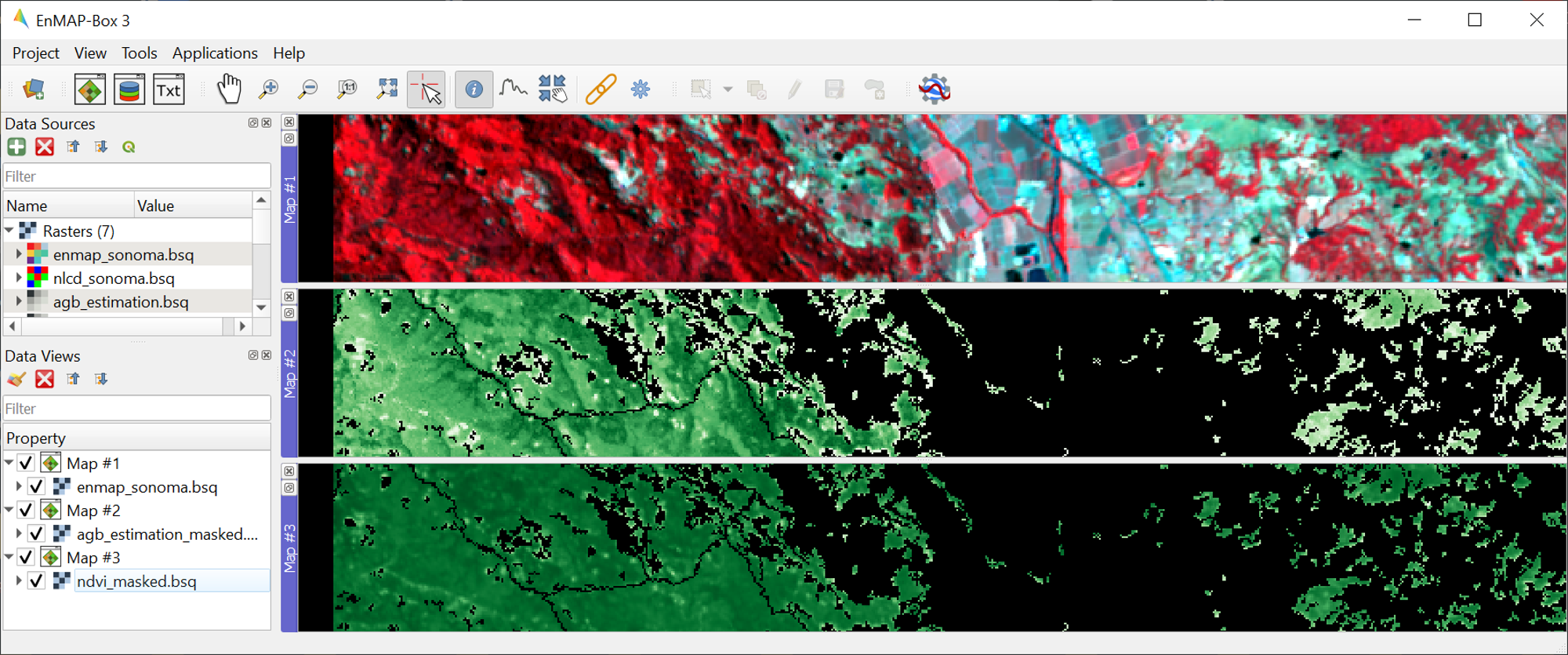
• Close all Map Views.
• Open an RGB composite of enmap_sonoma.bsq in Map #1.
• Display agb_estimation_masked.bsq and ndvi_masked.bsq in Map#2 and Map#3, respectively and use the Layer Properties to change the color ramp of both maps to white-green. Link all Map Views.

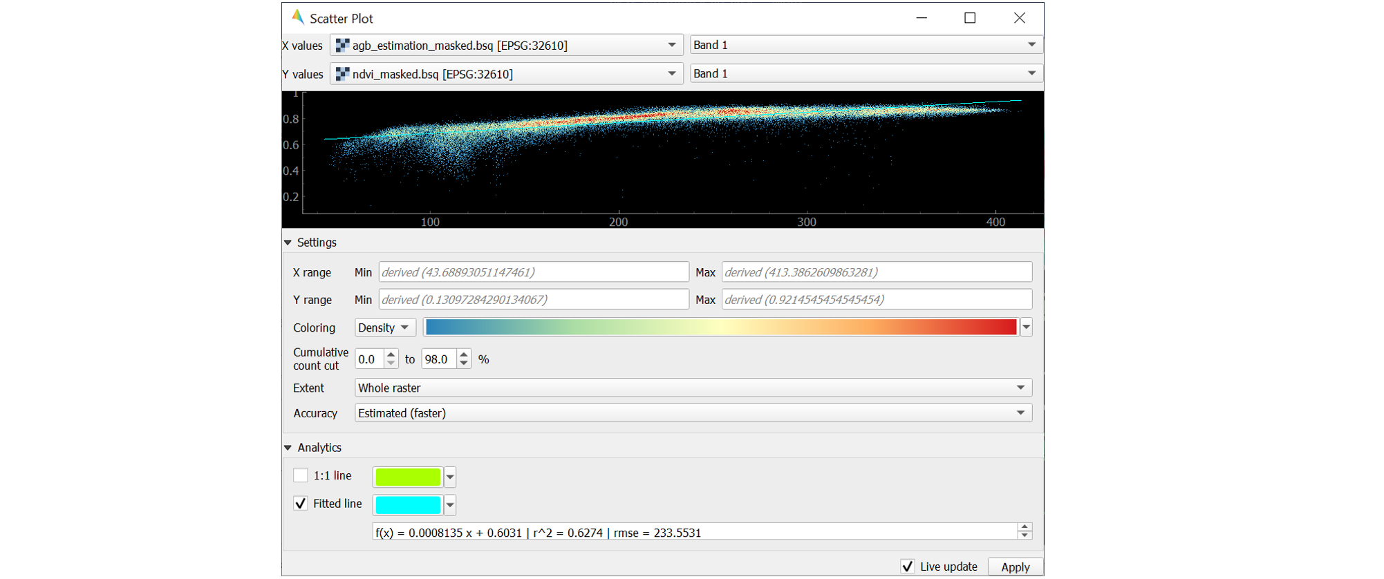
• To investigate the relationship between estimated AGB and NDVI, we will make use of the EnMAP-Box’s Scatter Plot tool. This is one of several tools integrated into the EnMAP-Box to support data visualization and assessment

• Open the Scatter Plot tool by going to Tools then selecting Scatter Plot.

  • Select agb_estimation_masked.bsq and Band 1 for specifying X values and ndvi_masked.bsq and Band 1 for specifying Y values. If a selected raster has multiple bands, you would specify the desired band from the dropdown.
  • Click on Apply to visualize the Scatter Plot.

• The Settings offer different options for visualizing the scatter plot.

  • You may change the Min and Max values, Coloring or Cumulative count cut options to improve your visualization.
  • Under Extent you may choose Current canvas or Whole raster to display data of the current map canvas only or to display all raster data. Choose Whole raster.
  • Under Accuracy you may choose to display Estimated or Actual. Actual will display all available data, while Estimated will only display a random subset. For large raster extents, Estimated is much faster, and for that reason is the default. Leave Accuracy as Estimated.
  • Click on Apply to update the Scatter Plot. If Live update is checked, visualization of the scatter plot will be automatically updated.

• The Analytics offers options to assess the relationship between x and y values.

  • The 1:1 line represents the linear 1:1 relationship between the two variables of the same unit if they were perfectly correlated.
  • The Fitted line represents the linear regression line fitted between the actual data from the two variables. The linear regression function, the coefficient of determination (r^2) and the Root Mean Squared Error (rmse) will be additionally displayed. Activate the Min-max line by checking the box to its left.

Learning Activities

Learning Activities

• C1: Why was it necessary to mask the AGB results?
• C2: What relationships can you see between AGB and NDVI? Do these relationships hold true if you look at the un-masked AGB and NDVI maps?
• C3: Given the relationships between AGB and NDVI, do you think NDVI could be used to map AGB? What limitations would you expect from such a model?

Additional Exercises

Learning Activities

• AE1: Use the Image Statistics tool in the Tools menu to look at the band statistics for the biomass predictions both with and without the tree mask applied.
• AE2: Because we randomly subsetted the training data prior to model training, the performance of the model has an element of uncertainty to it. To better understand this, rerun the regression workflow 3-5 times. Then use the ImageMath tool to calculate the average estimate and variance. How does running the regression in such an ensemble approach affect the results? What is the spatial pattern of variation in estimates?
• AE3: Rerun regression (Exercise B) using NDVI as the input rather than the hyperspectral imagery.