Glossary

This glossary gives an overview of how specific terms are used inside the EnMAP-Box.

All the terms that relate to GIS in general should be consistent with the terms given by the QGIS user manual and GUI. Because the EnMAP-Box integrates into the QGIS GUI, we try to not (as far as possible) contradict or redefine terminology.

All terms that relate to machine learning should be consistent with the definitions given by Scikit-Learn and the Scikit-Learn glossary, because we wildly crosslink into the Scikit-Learn docs!

Index with all Terms

Index

GIS and Remote Sensing

attribute

A synonym for field.

attribute table

A tabulated data table associated with a vector layer. Table columns and rows are referred to as fields and geographic features respectively.

attribute value

Refers to a single cell value inside the attribute table of a vector layer.

band

A raster layer is composed of one or multiple bands.

categorized layer

A categorized vector layer or categorized raster layer.

categorized raster layer

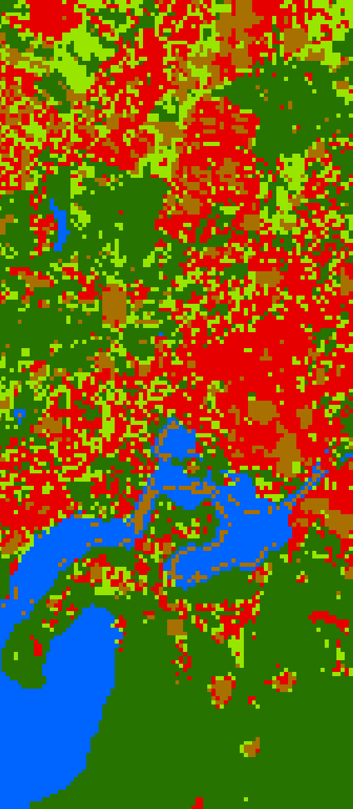
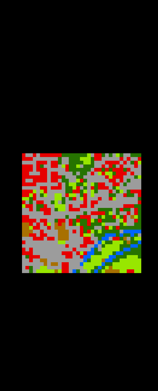
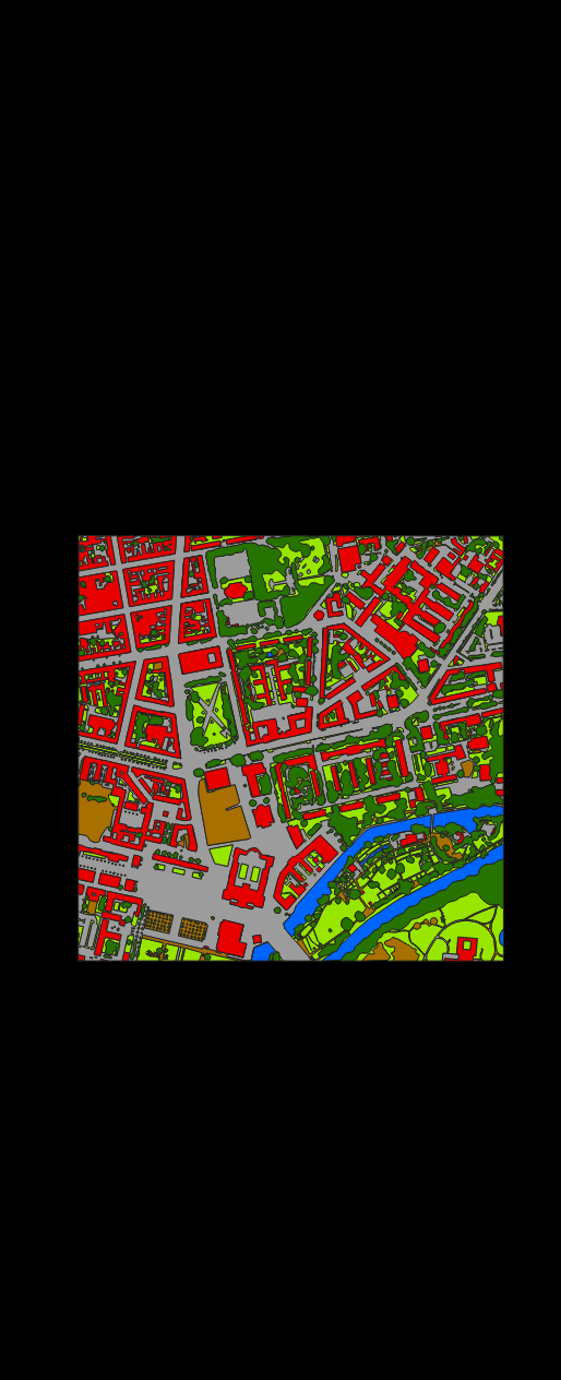
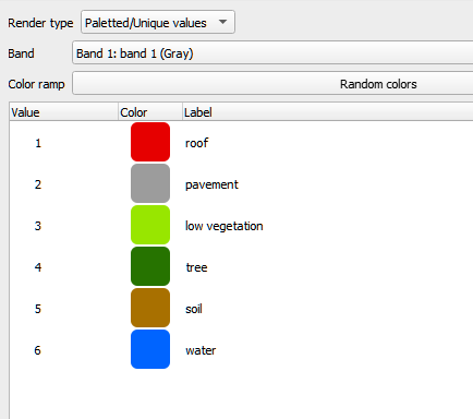
A raster layer styled with a Paletted/Unique values renderer. The renderer defines the band with category values and a list of named and colored categories. Styles are usually stored as QML sidecar files. Category values don’t have to be strictly consecutive.

categorized vector layer

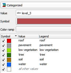
A vector layer styled with a Categorized renderer. The renderer defines the field storing the category values (numbers or strings; expressions not yet supported) and a list of named and colored categories. Styles are usually stored as QML sidecar files. Note that in case of numerical category values, the values don’t have to be strictly consecutive.

categorized spectral library

A spectral library that is also a categorized vector layer.

category

categories

A category has a value, a name and a color.

class

Synonym for category.

classification layer

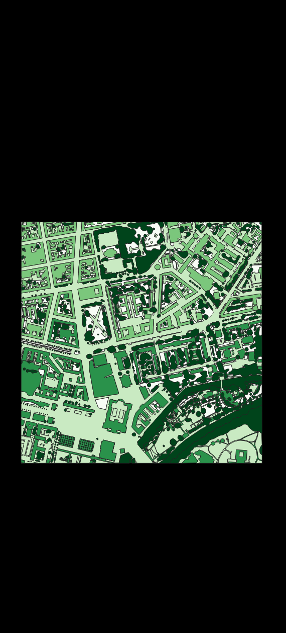
A categorized raster layer that is assumed to represent a mapping of a contiguous area.

Note that there is currently no equivalent term for a contiguous vector polygon layer. We may introduce it in the future as needed. For now we expect users to rasterize such a vector layer into a raster layer.

class probability layer

A multi-band raster layer, where the bands represent class probabilities (values between 0 and 1) for a set of categories.

class fraction layer

A multi-band raster layer, where the bands represent class cover fractions (values between 0 and 1) for a set of categories.

color

An rgb-color, hex-color or int-color specified by a red, green and blue component. Learn more here: https://htmlcolorcodes.com/

continuous-valued raster layer

A raster layer, where each band represents a continuous-valued variable.

Variable names are given by the raster band names. Variable colors are given by the PAMRasterBand/Metadata “color” item (optional).

continuous-valued vector layer

A vector layer styled with a Graduated or a Diagrams renderer. Styles are usually stored as QML sidecar files.

A Graduated renderer specifies a single field used as continuous-valued variable. Variable name is given by the field name and color is given by the symbol color.

TODO: screenshot for graduated renderer (see issue #1038)

A Diagrams renderer specifies multiple fields used as continuous-valued variables. Variable names and colors is given by assigned attribute names and colors.

TODO: screenshot for diagrams renderer (see issue #1038)

continuous-valued layer

A continuous-valued vector layer or continuous-valued raster layer.

TODO: update screenshot (see issue #1038)

continuous-valued spectral library

A spectral library that is also a continuous-valued vector layer.

TODO: update screenshot (see issues #1036 and #1038)

continuous-valued variable

A continuous-valued variable has a name and (optional) a color.

field

Refers to a single column inside the attribute table of a vector layer.

A synonym for attribute.

geographic feature

Refers to a single row inside the attribute table of a vector layer. In a vector layer, a geographic feature is a logical element defined by a point, polyline or polygon.

Note that in the context of GIS, the epithet “geographic” in “geographic feature” is usually skipped. In the context of EnMAP-Box, and machine learning in general, the term “feature” is used differently.

See feature for details.

grid

A raster layer defining the spatial extent, coordinate reference system and the pixel size.

hex-color

A color specified by a 6-digit hex-color string, where each color component is represented by a two digit hexadecimal number, e.g. red #FF0000, green #00FF00, blue #0000FF, black #000000, white #FFFFFF and grey #808080.

int-color

A color specified by a single integer between 0 and 256^3 - 1, which can also be represented as a hex-color.

labeled layer

A categorized layer or a continuous-valued layer.

layer

A vector layer or a raster layer.

layer style

The style of a layer can be defined in the Layer Styling panel and the Styling tab of the Layer Properties dialog. Some applications and algorithms take advantage of style information, e.g. for extracting category names and colors.

mask layer

A mask raster layer or mask vector layer.

mask raster layer

A raster layer interpreted as a binary mask. All no data (zero, if missing), inf and nan pixel evaluate to false, all other to true. Note that only the first band used by the renderer is considered.

mask vector layer

A vector layer interpreted as a binary mask. Areas covered by a geometry evaluate to true, all other to false.

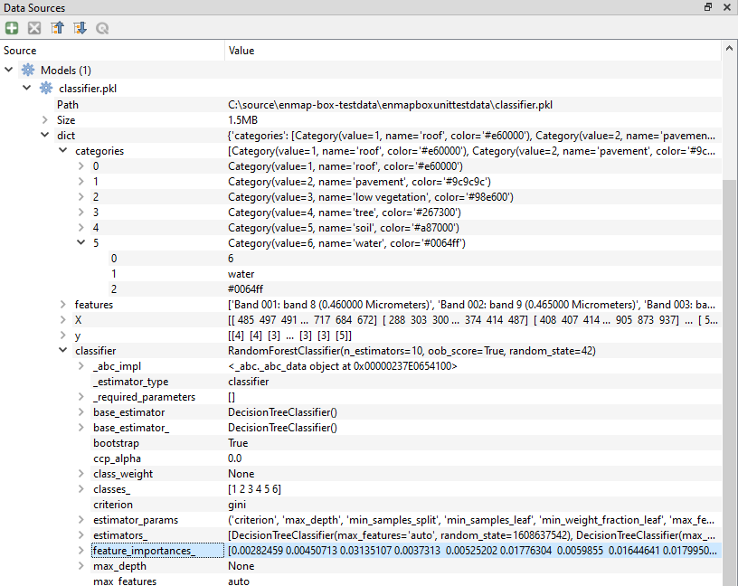
pickle file

A binary file ending on .pkl that contains a pickled Python object, usually a dictionary or list container. Pickle file content can be browsed via the EnMAP-Box Data Sources panel:

pixel profile

List of band values for a single pixel in a raster layer.

point layer

A vector layer with point geometries.

polygon layer

A vector layer with polygon geometries.

ployline layer

A vector layer with line geometries.

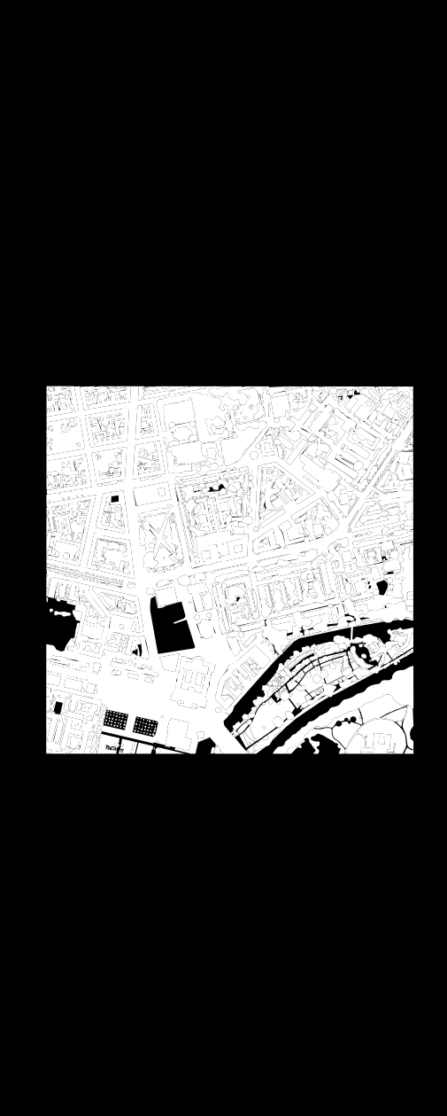
raster layer

Any raster file that can be opened in QGIS as QgsRasterLayer. Elsewhere known as an image.

regression layer

A continuous-valued raster layer that is assumed to represent a mapping of a contiguous area.

rgb-color

A color specified by a triplet of byte values (values between 0 and 255) representing the red, green and blue color components, e.g. red (255, 0, 0), green (0, 255, 0), blue (0, 0, 255), black (0, 0, 0), white (255, 255, 255) and grey (128, 128, 128).

RGB image

A 3-band byte raster layer with values ranging from 0 to 255.

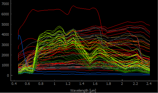
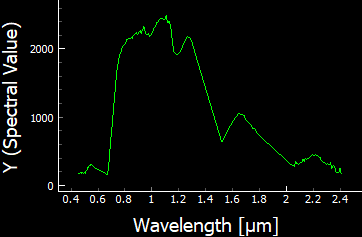
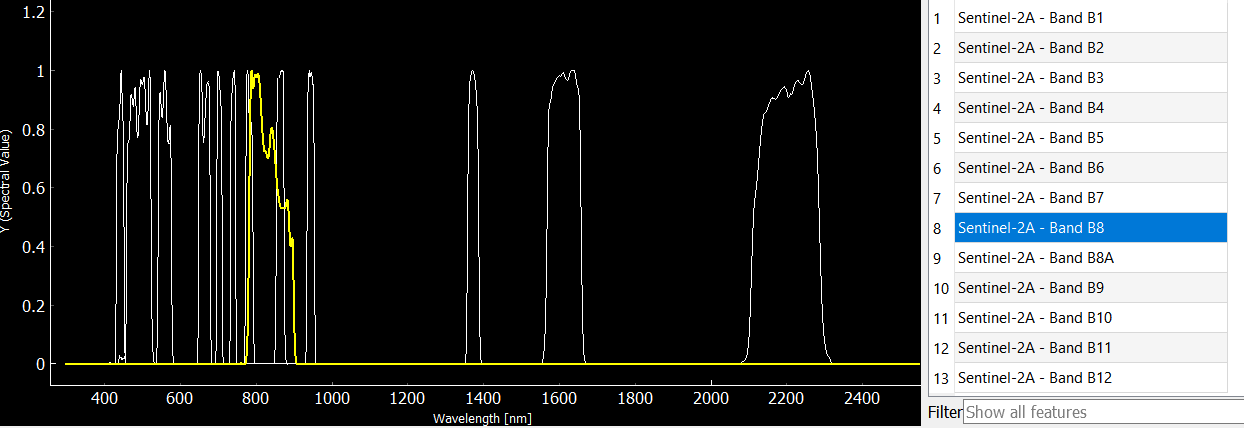
spectral band

A band inside a spectral raster layer. A spectral band represents a measurement for a region of the electromagnetic spectrum around a specific center wavelength. The region is typically described by a spectral response function.

spectral library

A vector layer with at least one text, JSON or binary field that is designated to a Spectral Profiles editor. Such Spectral Profile fields can contain profile data. Additional metadata can be stored like in any other vector layer, e.g. in text and numeric fields.

Using a vector layer with multiple Spectral Profile fields, it possible to link different profiles to the same geographic feature, e.g. a white reference profile to a field spectrometer profile relating to the same spatial position.

A single profile is represented by a dictionary of the following values:

• y: list of y values, required (e.g. surface reflectance)

• x: list of x values, optional (e.g. wavelength)

• xUnit: x value units, optional (e.g. nanometers)

• yUnit: y value units, optional (e.g. ???)

• bbl: optional list of bad band multiplier values

Depending on the selected data type of the spectral profile field, the dictionary is stored as plain JSON text or binarized JSON object.

See enmapbox.qgispluginsupport.qps.speclib.core.SpectralLibraryUtils for details.

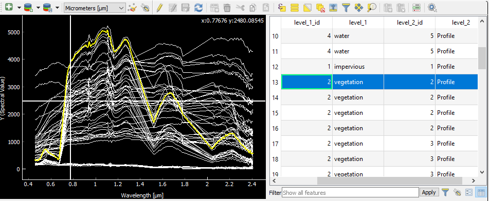
spectral profile

A pixel profile in a spectral raster layer or a profile in a spectral library.

spectral raster layer

A raster layer with proper wavelength and wavelength units metadata, where the individual bands (i.e. spectral bands) represent measurements across the electromagnetic spectrum. The measurement vector of a single pixel is called a spectral profile)

spectral response function

The spectral response describes the sensitivity of a sensor to optical radiation of different wavelengths. In hyperspectral remote sensing, the spectral response function is often described by a single full-width-at-half-maximum value.

spectral response function library

A spectral library, where each profile represents the spectral response function of a spectral band.

stratification layer

A classification layer that is used to stratify an area into distinct subareas.

stratum

strata

A category of a classifcation layer that is used as a stratification layer. Conceptually, a stratum can be seen as a binary mask with all pixels inside the stratum evaluating to True and all other pixels evaluating to False.

table

A vector layer with (potentially) missing geometry.

Note that in case of missing geometry, the vector layer icon looks like a table and layer styling is disabled.

vector feature

Synonym for geographic feature.

vector layer

Any vector file that can be opened in QGIS as QgsVectorLayer.

Raster Metadata

Introduction

Raster metadata management is mainly based on the GDAL PAM (Persistent Auxiliary Metadata) model. Depending on the type of metadata, managing specific metadata item in the GUI or programmatically can differ. Details are explained in the specific term descriptions below.

In the GUI, most of the metadata items can be inspected in the Layer Properties dialog, under GDAL Metadata.

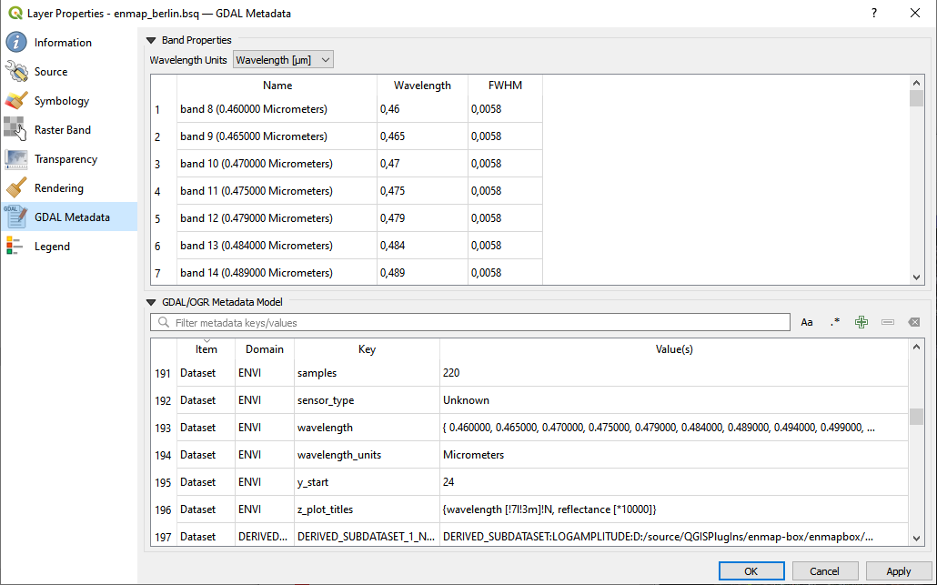
Alternatively, metadata can be managed inside a standard text editor, by opening the GDAL PAM *.aux.xml sidecar file. If the PAM file not already exists, you can create it manually, but usually, it is also created, when a raster file is opened inside QGIS. Here is an excerpt of the enmap_berlin.bsq.aux.xml PAM file:

<PAMDataset>
  <Metadata domain="ENVI">
    <MDI key="band_names">{band 8, band 9, band 10, band 11, band 12, band 13, band 14, band 15, band 16, band 17, band 18, band 19, band 20, band 21, band 22, band 23, band 24, band 25, band 26, band 27, band 28, band 29, band 30, band 31, band 32, band 33, band 34, band 35, band 36, band 37, band 38, band 39, band 40, band 41, band 42, band 43, band 44, band 45, band 46, band 47, band 48, band 49, band 50, band 51, band 52, band 53, band 54, band 55, band 56, band 57, band 58, band 59, band 60, band 61, band 62, band 63, band 64, band 65, band 66, band 67, band 68, band 69, band 70, band 71, band 72, band 73, band 74, band 75, band 76, band 77, band 91, band 92, band 93, band 94, band 95, band 96, band 97, band 98, band 99, band 100, band 101, band 102, band 103, band 104, band 105, band 106, band 107, band 108, band 109, band 110, band 111, band 112, band 113, band 114, band 115, band 116, band 117, band 118, band 119, band 120, band 121, band 122, band 123, band 124, band 125, band 126, band 127, band 144, band 145, band 146, band 147, band 148, band 149, band 150, band 151, band 152, band 153, band 154, band 155, band 156, band 157, band 158, band 159, band 160, band 161, band 162, band 163, band 164, band 165, band 166, band 167, band 168, band 195, band 196, band 197, band 198, band 199, band 200, band 201, band 202, band 203, band 204, band 205, band 206, band 207, band 208, band 209, band 210, band 211, band 212, band 213, band 214, band 215, band 216, band 217, band 218, band 219, band 220, band 221, band 222, band 223, band 224, band 225, band 226, band 227, band 228, band 229, band 230, band 231, band 232, band 233, band 234, band 235, band 236, band 237, band 238, band 239}</MDI>
    <MDI key="fwhm">{ 0.005800, 0.005800, 0.005800, 0.005800, 0.005800, 0.005800, 0.005800, 0.005800, 0.005800, 0.005800, 0.005900, 0.005900, 0.006000, 0.006000, 0.006100, 0.006100, 0.006200, 0.006200, 0.006300, 0.006400, 0.006400, 0.006500, 0.006600, 0.006600, 0.006700, 0.006800, 0.006900, 0.006900, 0.007000, 0.007100, 0.007200, 0.007300, 0.007300, 0.007400, 0.007500, 0.007600, 0.007700, 0.007800, 0.007900, 0.007900, 0.008000, 0.008100, 0.008200, 0.008300, 0.008400, 0.008400, 0.008500, 0.008600, 0.008700, 0.008700, 0.008800, 0.008900, 0.008900, 0.009000, 0.009100, 0.009100, 0.009200, 0.009300, 0.009300, 0.009400, 0.009400, 0.009500, 0.009500, 0.009600, 0.009600, 0.009600, 0.009600, 0.009700, 0.009700, 0.009700, 0.011800, 0.011900, 0.012100, 0.012200, 0.012400, 0.012500, 0.012700, 0.012800, 0.012900, 0.013100, 0.013200, 0.013300, 0.013400, 0.013500, 0.013600, 0.013700, 0.013800, 0.013900, 0.014000, 0.014000, 0.014100, 0.014100, 0.014200, 0.014200, 0.014300, 0.014300, 0.014300, 0.014400, 0.014400, 0.014400, 0.014400, 0.014400, 0.014400, 0.014400, 0.014400, 0.014400, 0.014400, 0.013700, 0.013600, 0.013600, 0.013500, 0.013500, 0.013400, 0.013400, 0.013300, 0.013200, 0.013200, 0.013100, 0.013100, 0.013000, 0.012900, 0.012900, 0.012800, 0.012800, 0.012700, 0.012700, 0.012600, 0.012500, 0.012500, 0.012400, 0.012400, 0.012300, 0.010900, 0.010800, 0.010800, 0.010700, 0.010700, 0.010600, 0.010600, 0.010500, 0.010500, 0.010400, 0.010400, 0.010400, 0.010300, 0.010300, 0.010200, 0.010200, 0.010100, 0.010100, 0.010100, 0.010000, 0.010000, 0.009900, 0.009900, 0.009900, 0.009800, 0.009800, 0.009700, 0.009700, 0.009700, 0.009600, 0.009600, 0.009600, 0.009500, 0.009500, 0.009400, 0.009400, 0.009400, 0.009300, 0.009300, 0.009300, 0.009200, 0.009200, 0.009100, 0.009100, 0.009100}</MDI>
    <MDI key="wavelength">{ 0.460000, 0.465000, 0.470000, 0.475000, 0.479000, 0.484000, 0.489000, 0.494000, 0.499000, 0.503000, 0.508000, 0.513000, 0.518000, 0.523000, 0.528000, 0.533000, 0.538000, 0.543000, 0.549000, 0.554000, 0.559000, 0.565000, 0.570000, 0.575000, 0.581000, 0.587000, 0.592000, 0.598000, 0.604000, 0.610000, 0.616000, 0.622000, 0.628000, 0.634000, 0.640000, 0.646000, 0.653000, 0.659000, 0.665000, 0.672000, 0.679000, 0.685000, 0.692000, 0.699000, 0.706000, 0.713000, 0.720000, 0.727000, 0.734000, 0.741000, 0.749000, 0.756000, 0.763000, 0.771000, 0.778000, 0.786000, 0.793000, 0.801000, 0.809000, 0.817000, 0.824000, 0.832000, 0.840000, 0.848000, 0.856000, 0.864000, 0.872000, 0.880000, 0.888000, 0.896000, 0.915000, 0.924000, 0.934000, 0.944000, 0.955000, 0.965000, 0.975000, 0.986000, 0.997000, 1.007000, 1.018000, 1.029000, 1.040000, 1.051000, 1.063000, 1.074000, 1.086000, 1.097000, 1.109000, 1.120000, 1.132000, 1.144000, 1.155000, 1.167000, 1.179000, 1.191000, 1.203000, 1.215000, 1.227000, 1.239000, 1.251000, 1.263000, 1.275000, 1.287000, 1.299000, 1.311000, 1.323000, 1.522000, 1.534000, 1.545000, 1.557000, 1.568000, 1.579000, 1.590000, 1.601000, 1.612000, 1.624000, 1.634000, 1.645000, 1.656000, 1.667000, 1.678000, 1.689000, 1.699000, 1.710000, 1.721000, 1.731000, 1.742000, 1.752000, 1.763000, 1.773000, 1.783000, 2.044000, 2.053000, 2.062000, 2.071000, 2.080000, 2.089000, 2.098000, 2.107000, 2.115000, 2.124000, 2.133000, 2.141000, 2.150000, 2.159000, 2.167000, 2.176000, 2.184000, 2.193000, 2.201000, 2.210000, 2.218000, 2.226000, 2.234000, 2.243000, 2.251000, 2.259000, 2.267000, 2.275000, 2.283000, 2.292000, 2.300000, 2.308000, 2.315000, 2.323000, 2.331000, 2.339000, 2.347000, 2.355000, 2.363000, 2.370000, 2.378000, 2.386000, 2.393000, 2.401000, 2.409000}</MDI>
    <MDI key="wavelength_units">Micrometers</MDI>
    ...
  </Metadata>
  <PAMRasterBand band="1">
    <Description>band 8 (0.460000 Micrometers)</Description>
    <NoDataValue>-9.90000000000000E+01</NoDataValue>
    <Metadata>
      <MDI key="wavelength">0.460000</MDI>
      <MDI key="wavelength_units">Micrometers</MDI>
    </Metadata>
  </PAMRasterBand>

  <PAMRasterBand band="1">
    ...
  </PAMRasterBand>

  ...

</PAMDataset>

For managing metadata programmatically, you can mostly use the GDAL API classes gdal.Datset and gdal.Band, or the EnMAP-Box API classes enmapboxprocessing.rasterreader.RasterReader and enmapboxprocessing.rasterreader.RasterWriter.

Warning

If you want to edit metadata in an editor or programmatically, be sure to first close the associated raster layer inside QGIS. Otherwise, QGIS will overwrite your changes again.

To examplify the API usage, we assume the following namespace setup throughout the rest of this section:

from osgeo import gdal
from enmapboxprocessing.rasterreader import RasterReader
from enmapboxprocessing.rasterwriter import RasterWriter
from enmapbox.exampledata import enmap

# use enmap_berlin.bsq raster layer as example dataset
dataset: gdal.Dataset = gdal.Open(enmap)
raster = RasterReader(enmap)

# assume we have a newly created gdal.Dataset object in update mode
newDataset: gdal.Dataset
newRaster = RasterWriter(newDataset)

# for band-wise interactions, we just use the first band
bandNo = 1

bad band

bad band list

bad band multiplier

bbl

The bad band multiplier value is indicating whether a band is usable (1) or not (0).

This information is derived from PAM/Band/Default/bbl. If that is undefined, it is derived by indexing the ENVI bad bands list from PAM/Dataset/ENVI/bbl. If that is also undefined, it is assumed, that the band is usable (i.e. value=1):

# get
>>>dataset.GetRasterBand(bandNo).GetMetadataItem('bbl')  # isn't sufficient in this case
>>>dataset.GetMetadataItem('bbl', 'ENVI')  # also not sufficient
>>>raster.badBandMultiplier(bandNo)  # this will correctly resolve the bad band multiplier
None
None
1

# set
>>>newDataset.GetRasterBand(bandNo).SetMetadataItem('bbl', '1')  # set for single band
>>>newDataset.SetMetadataItem('bbl', '{1, ...., 1}', 'ENVI')  # set for all bands at once
>>>newRaster.setBadBandMultiplier(1, bandNo)  # set for single band

band description

band name

The name of a band.

Usage example:

# get
>>>dataset.GetRasterBand(bandNo).GetDescription()
>>>raster.bandName(bandNo)
band 8 (0.460000 Micrometers)
band 8 (0.460000 Micrometers)

# set
>>>newDataset.GetRasterBand(bandNo).SetDescription('my band name')
>>>newRaster.setBandName('my band name', bandNo)

center wavelength

A synonym for wavelength.

fwhm

full-width-at-half-maximum

The full-width-half-maximum (FWHM) value of a spectral band is approximating the spectral response function as a normal distribution with a sigma = FWHM / 2.355. Units should be the same as those used for wavelength and set in the wavelength units item.

This information is derived from PAM/Band/Default/fwhm. If that is undefined, it is derived by indexing the ENVI fwhm list from PAM/Dataset/ENVI/fwhm:

# get
>>>dataset.GetRasterBand(bandNo).GetMetadataItem('fwhm')  # isn't sufficient in this case
>>>text = dataset.GetMetadataItem('fwhm', 'ENVI')  # this gives just a string with values for all bands
>>>text
>>>float(text.strip('{}').split(',')[bandNo - 1])  # extra processing required to unpack the band FWHM
>>>raster.badBandMultiplier(bandNo)  # in Nanometers (the default)
>>>raster.badBandMultiplier(bandNo, 'Micrometers')  #  in user-defined units
None
{ 0.005800, 0.005800, 0.005800, 0.005800, 0.005800, 0.005800, 0.005800, 0.005800, 0.005800, 0.005800, 0.005900, 0.005900, 0.006000, 0.006000, 0.006100, 0.006100, 0.006200, 0.006200, 0.006300, 0.006400, 0.006400, 0.006500, 0.006600, 0.006600, 0.006700, 0.006800, 0.006900, 0.006900, 0.007000, 0.007100, 0.007200, 0.007300, 0.007300, 0.007400, 0.007500, 0.007600, 0.007700, 0.007800, 0.007900, 0.007900, 0.008000, 0.008100, 0.008200, 0.008300, 0.008400, 0.008400, 0.008500, 0.008600, 0.008700, 0.008700, 0.008800, 0.008900, 0.008900, 0.009000, 0.009100, 0.009100, 0.009200, 0.009300, 0.009300, 0.009400, 0.009400, 0.009500, 0.009500, 0.009600, 0.009600, 0.009600, 0.009600, 0.009700, 0.009700, 0.009700, 0.011800, 0.011900, 0.012100, 0.012200, 0.012400, 0.012500, 0.012700, 0.012800, 0.012900, 0.013100, 0.013200, 0.013300, 0.013400, 0.013500, 0.013600, 0.013700, 0.013800, 0.013900, 0.014000, 0.014000, 0.014100, 0.014100, 0.014200, 0.014200, 0.014300, 0.014300, 0.014300, 0.014400, 0.014400, 0.014400, 0.014400, 0.014400, 0.014400, 0.014400, 0.014400, 0.014400, 0.014400, 0.013700, 0.013600, 0.013600, 0.013500, 0.013500, 0.013400, 0.013400, 0.013300, 0.013200, 0.013200, 0.013100, 0.013100, 0.013000, 0.012900, 0.012900, 0.012800, 0.012800, 0.012700, 0.012700, 0.012600, 0.012500, 0.012500, 0.012400, 0.012400, 0.012300, 0.010900, 0.010800, 0.010800, 0.010700, 0.010700, 0.010600, 0.010600, 0.010500, 0.010500, 0.010400, 0.010400, 0.010400, 0.010300, 0.010300, 0.010200, 0.010200, 0.010100, 0.010100, 0.010100, 0.010000, 0.010000, 0.009900, 0.009900, 0.009900, 0.009800, 0.009800, 0.009700, 0.009700, 0.009700, 0.009600, 0.009600, 0.009600, 0.009500, 0.009500, 0.009400, 0.009400, 0.009400, 0.009300, 0.009300, 0.009300, 0.009200, 0.009200, 0.009100, 0.009100, 0.009100}
0.0058
5.8
0.0058

# set
>>>newDataset.GetRasterBand(bandNo).SetMetadataItem('fwhm', '0.0058')  # set FWHM for single band
>>>newDataset.GetRasterBand(bandNo).SetMetadataItem('wavelength_units', 'Micrometers')  # also set the units
>>>newDataset.SetMetadataItem('fwhm', '{0.0058, ..., 0.0091}', 'ENVI')  # set FWHM for all bands at once
>>>newDataset.SetMetadataItem('wavelength_units', 'Micrometers', 'ENVI')  # also set the units
>>>newRaster.setFwhm(5.8, bandNo)  # set single band FWHM in Nanometers
>>>newRaster.setFwhm(0.0058, bandNo, 'Micrometers')  # set single band FWHM in user-defined units

no data value

The no data value of a band.

Usage example:

# get
>>>dataset.GetRasterBand(bandNo).GetNoDataValue()
>>>raster.noDataValue(bandNo)
>>>raster.noDataValue()  # if bandNo is skipped, it defaults to the first band
-99.0
-99.0
-99.0

# set
newDataset.GetRasterBand(bandNo).SetNoDataValue(-9999)
newRaster.setNoDataValue(-9999, bandNo)
newRaster.setNoDataValue(-9999)  # if bandNo is skipped, the no data value is applied to all bands

wavelength

The center wavelength value of a band. Units should be the same as those used for the fwhm and set in the wavelength units item.

This information is derived from PAM/Band/Default/wavelength. If that is undefined, it is derived by indexing the ENVI wavelength list from PAM/Dataset/ENVI/wavelength:

# get
>>>dataset.GetRasterBand(bandNo).GetMetadataItem('wavelength')  # this works, because the GDAL ENVI driver assigns those on-the-fly
>>>text = dataset.GetMetadataItem('fwhm', 'ENVI')  # this gives just a string with values for all bands
>>>text
>>>float(text.strip('{}').split(',')[bandNo - 1])  # extra processing required to unpack the band wavelength
>>>raster.wavelength(bandNo)  # in Nanometers (the default)
>>>raster.wavelength(bandNo, 'Micrometers')  #  in user-defined units
0.460000
{ 0.460000, 0.465000, 0.470000, 0.475000, 0.479000, 0.484000, 0.489000, 0.494000, 0.499000, 0.503000, 0.508000, 0.513000, 0.518000, 0.523000, 0.528000, 0.533000, 0.538000, 0.543000, 0.549000, 0.554000, 0.559000, 0.565000, 0.570000, 0.575000, 0.581000, 0.587000, 0.592000, 0.598000, 0.604000, 0.610000, 0.616000, 0.622000, 0.628000, 0.634000, 0.640000, 0.646000, 0.653000, 0.659000, 0.665000, 0.672000, 0.679000, 0.685000, 0.692000, 0.699000, 0.706000, 0.713000, 0.720000, 0.727000, 0.734000, 0.741000, 0.749000, 0.756000, 0.763000, 0.771000, 0.778000, 0.786000, 0.793000, 0.801000, 0.809000, 0.817000, 0.824000, 0.832000, 0.840000, 0.848000, 0.856000, 0.864000, 0.872000, 0.880000, 0.888000, 0.896000, 0.915000, 0.924000, 0.934000, 0.944000, 0.955000, 0.965000, 0.975000, 0.986000, 0.997000, 1.007000, 1.018000, 1.029000, 1.040000, 1.051000, 1.063000, 1.074000, 1.086000, 1.097000, 1.109000, 1.120000, 1.132000, 1.144000, 1.155000, 1.167000, 1.179000, 1.191000, 1.203000, 1.215000, 1.227000, 1.239000, 1.251000, 1.263000, 1.275000, 1.287000, 1.299000, 1.311000, 1.323000, 1.522000, 1.534000, 1.545000, 1.557000, 1.568000, 1.579000, 1.590000, 1.601000, 1.612000, 1.624000, 1.634000, 1.645000, 1.656000, 1.667000, 1.678000, 1.689000, 1.699000, 1.710000, 1.721000, 1.731000, 1.742000, 1.752000, 1.763000, 1.773000, 1.783000, 2.044000, 2.053000, 2.062000, 2.071000, 2.080000, 2.089000, 2.098000, 2.107000, 2.115000, 2.124000, 2.133000, 2.141000, 2.150000, 2.159000, 2.167000, 2.176000, 2.184000, 2.193000, 2.201000, 2.210000, 2.218000, 2.226000, 2.234000, 2.243000, 2.251000, 2.259000, 2.267000, 2.275000, 2.283000, 2.292000, 2.300000, 2.308000, 2.315000, 2.323000, 2.331000, 2.339000, 2.347000, 2.355000, 2.363000, 2.370000, 2.378000, 2.386000, 2.393000, 2.401000, 2.409000}
0.46
460.0
0.46

# set
>>>newDataset.GetRasterBand(bandNo).SetMetadataItem('wavelength', '0.46')  # set wavelength for single band
>>>newDataset.GetRasterBand(bandNo).SetMetadataItem('wavelength_units', 'Micrometers')  # also set the units
>>>newDataset.SetMetadataItem('fwhm', '{0.46, ..., 2.409}', 'ENVI')  # set wavelength for all bands at once            >>>newDataset.SetMetadataItem('wavelength_units', 'Micrometers', 'ENVI')  # also set the units
>>>newRaster.setWavelength(460, bandNo)  # set single band wavelength in Nanometers
>>>newRaster.setWavelength(0.46, bandNo, 'Micrometers')  # set single band wavelength in user-defined units

wavelength units

The wavelength units of a band. Valid units are Micrometers, um, Nanometers, nm.

This information is derived from PAM/Band/Default/wavelength_units. If that is undefined, it is derived from PAM/Dataset/ENVI/wavelength_units:

# get
>>>dataset.GetRasterBand(bandNo).GetMetadataItem('wavelength_units')  # this works, because the GDAL ENVI driver assigns those on-the-fly
>>>dataset.GetMetadataItem('wavelength_units', 'ENVI')
>>>raster.wavelengthUnits(bandNo)
Micrometers
Micrometers
Micrometers

# set
>>>newDataset.GetRasterBand(bandNo).SetMetadataItem('wavelength_units', 'Micrometers')  # set for single band
>>>newDataset.SetMetadataItem('wavelength_units', 'Micrometers', 'ENVI')  # set for the dataset

Note that when using the RasterWriter for setting wavelength or fwhm information, the wavelength units are also correctly specified at the same time.

Machine Learning

EnMAP-Box provides nearly all of it’s machine learning related functionality by using Scikit-Learn in the background. So we decided to also adopt related terminology and concepts as far as possible, while still retaining the connection to GIS and remote sensing in the broader context of being a QGIS plugin. Most of the following definitions are directly taken from the Scikit-Learn glossary as is, and only expanded if necessary.

classification

The process of identifying which category an object belongs to.

classifier

A supervised estimator with a finite set of discrete possible output values.

clusterer

An unsupervised estimator with a finite set of discrete output values.

clustering

The process of automatic grouping of similar objects into sets.

cross-validation

The training dataset is split into k smaller sets and the following procedure is followed for each of the k “folds”:

• a model is trained using k-1 of the folds as training dataset

• the resulting model is used to predict the targets of the remaining part of the dataset

The performance can now be calculated from the predictions for the whole training dataset.

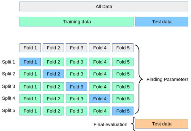
This approach can be computationally expensive, but does not waste too much data (as is the case when fixing an arbitrary validation set), which is a major advantage in problems where the number of samples is very small.

dataset

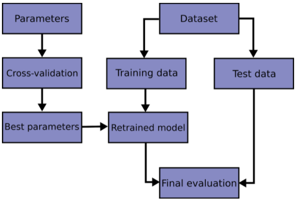
A dataset is a complete representation of a learning problem, combining feature data X and target data y. Datasets are often split into sub-datasets. One common splitting technique is the train-test split, where a part of the dataset is held out as a so-called training dataset used for fitting the estimator and another part is held out as a test dataset used for a final evaluation.

When evaluating different settings (i.e. hyperparameters) for an estimator, yet another part of the dataset can be held out as a so-called validation dataset. Training proceeds on the training dataset, best parameters are found by evaluating against the validation dataset, and final evaluation can be done on the test dataset. Holding out a validation datase can be avoided by using cross-validation for hyperparameter tuning.

estimator

An object which manages the estimation of a model. The model is estimated as a deterministic function.

evaluation metric

Evaluation metrics give a measure of how well a model (e.g. a classifier or regressor) performs.

See also https://scikit-learn.org/stable/modules/model_evaluation

feature

feature vector

In QGIS and other GIS, the term feature is well defined as a logical element defined by a point, polyline or polygon inside a vector layer. In the context of the EnMAP-Box, we refere to it as geographic feature.

In machine learning, a feature is a component in a so-called feature vector, which is a list of numeric quantities representing a sample in a dataset. A set of samples with feature data X and associated target data y or Y form a dataset.

Elsewhere features are known as attributes, predictors, regressors, or independent variables. Estimators assume that features are numeric, finite and not missing. n_features indicates the number of features in a dataset.

n_features

The number of features in a dataset.

n_outputs

The number of outputs in a dataset.

n_samples

The number of samples in a dataset.

n_targets

Synonym for n_outputs.

output

Individual scalar/categorical variables per sample in the target.

Also called responses, tasks or targets.

regression

The process of predicting a continuous-valued attribute associated with an object.

regressor

A supervised estimator with continuous output values.

sample

We usually use this term as a noun to indicate a single feature vector.

Elsewhere a sample is called an instance, data point, or observation. n_samples indicates the number of samples in a dataset, being the number of rows in a data array X.

target

The dependent variable in supervised learning, passed as y to an estimator’s fit method.

Also known as dependent variable, outcome variable, response variable, ground truth or label.

test dataset

The dataset used for final evaluation.

training dataset

The dataset used for training.

transformer

An estimator that transforms the input, usually only feature data X, into some transformed space (conventionally notated as Xt).

validation dataset

The dataset used for finding best parameters (i.e. hyperparameter tuning).

X

Denotes data that is observed at training and prediction time, used as independent variables in learning. The notation is uppercase to denote that it is ordinarily a matrix.

y

Y

Denotes data that may be observed at training time as the dependent variable in learning, but which is unavailable at prediction time, and is usually the target of prediction. The notation may be uppercase to denote that it is a matrix, representing multi-output targets, for instance; but usually we use y and sometimes do so even when multiple outputs are assumed.