Once you successfully installed the EnMAP-Box, you can access the plugin via the icon
in the QGIS toolbar or via Raster ‣ EnMAP-Box from the menubar.
Furthermore, the EnMAP-Box Processing Algorithms provider is available in the Processing Toolbox.
Fig. 5 The EnMAP-Box button in the QGIS Toolbar interface
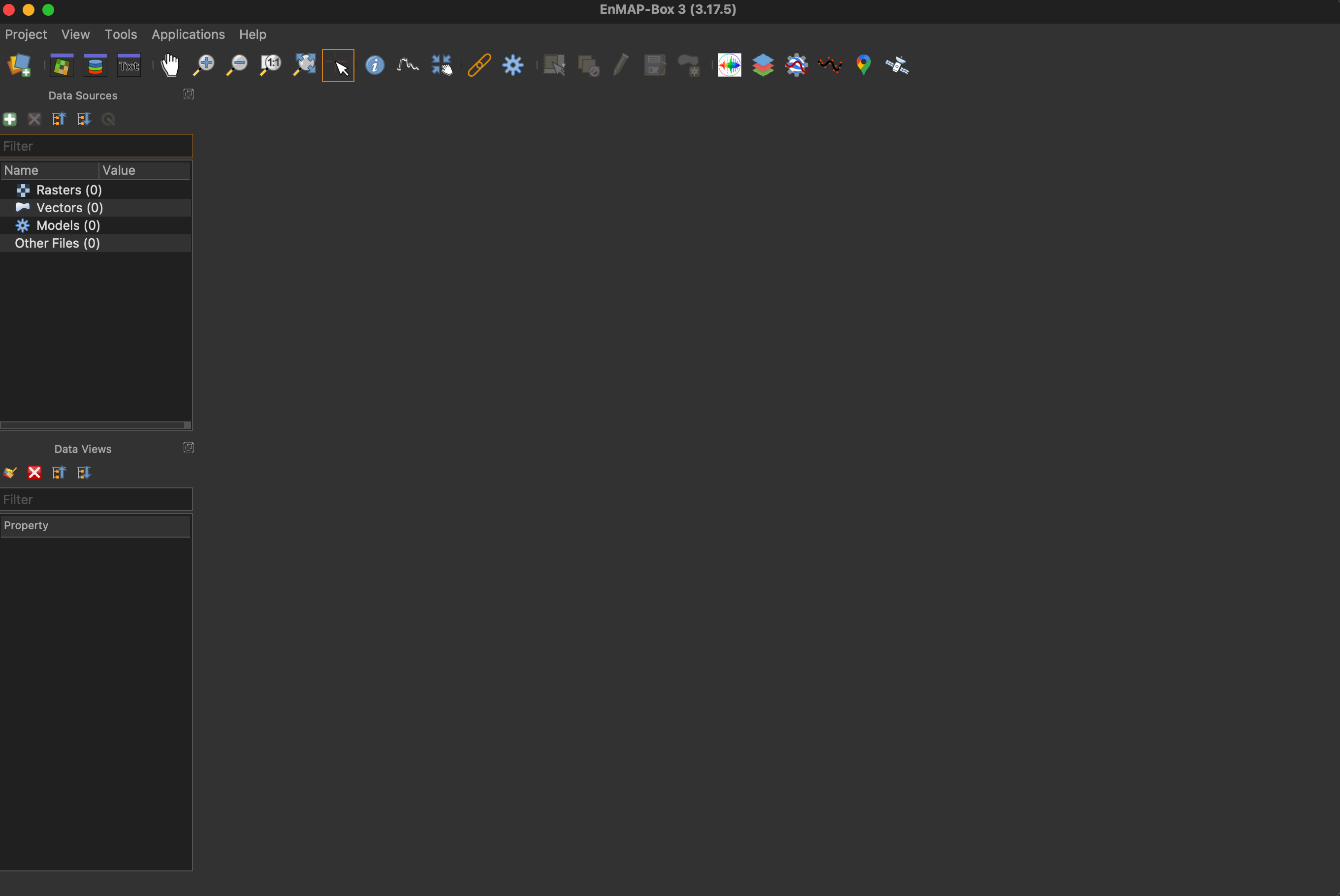
Fig. 6 The Graphical User Interface (GUI) of the EnMAP-Box on first open
Tip
Have a look at the User Manual for a detailed description of the GUI.
You can load an example dataset into your project by selecting Project ‣ Add Example Data in the menu bar.
On a fresh installation you will be asked to download the dataset, confirm with OK.
The data will be added automatically into a single map view and will be listed in the Data Sources panel as well.
By default the example data is loaded into a single map view. Let’s rearrange those for better visualization and in order
to get to know the GUI functionalities:
Click the Open a map view button to add a second map view. This view will appear below the
first map view (Map #1).
We want to arrange the windows so that they are next to each other (horizontally): Click and hold on to the blue area of
Map #2 and drag it to the right of Map #1 (see figure below). The translucent blue rectangle
indicates where the map window will be docked once you stop holding the left mouse button.
In the Map #1 list in the Data Views panel, select aerial_potsdam.tif and drag the
layer into Map #2 (you can drag them directly into the map view or the respective menu item under Data Views).
In the next step we link both map views, so that zoom and center are synchronized between both:
Click the button or go to View ‣ Set Map Linking and select
Link map scale and center.
Move the map (using or holding the mouse wheel ) and notice how both map views are synchronized now.
Now we want to change the RGB representation of the enmap_potsdam.tif image:
In the Data Views panel click the Open Raster Layer Styling button, which will open
a new panel. Here you can quickly change the renderer (e.g., singleband gray, RGB) and the band(s) visualized. You can
do so manually using the slider or by selecting the buttons with predefined wavelength regions based on Sentinel-2 (e.g.
G = Green, N = Near infrared).
The raster layer needs to have wavelength information for the latter to work!
In the RGB tab, look for Predefined and click on the dropdown menu . You will find several band
combination presets. Select Colour infrared.
Fig. 7 Raster Layer Styling panel with selected Color infrared preset
Try out other renderers and band combinations!
Tip
Once you selected/activated the slider (i.e., clicked on it) you can use the arrow keys ←/→ to
switch back and forth between bands!
In this section we will use a processing algorithm from the EnMAP-Box algorithm provider. The EnMAP-Box adds more than
180 Processing Algorithms to the QGIS processing framework. Their scope ranges from general tasks, e.g. file type
conversions or data import to specific applications like machine learning.
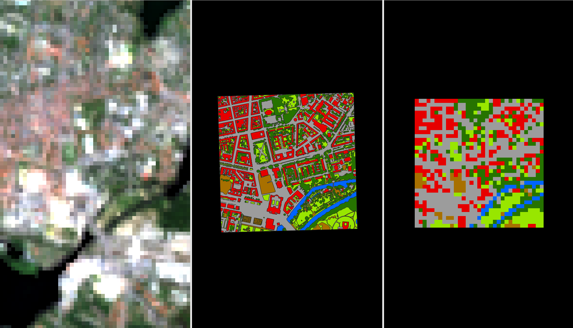
In this example we are converting a polygon dataset with information on different landcover types into a
classification raster, i.e., we are going to rasterize the vector dataset.
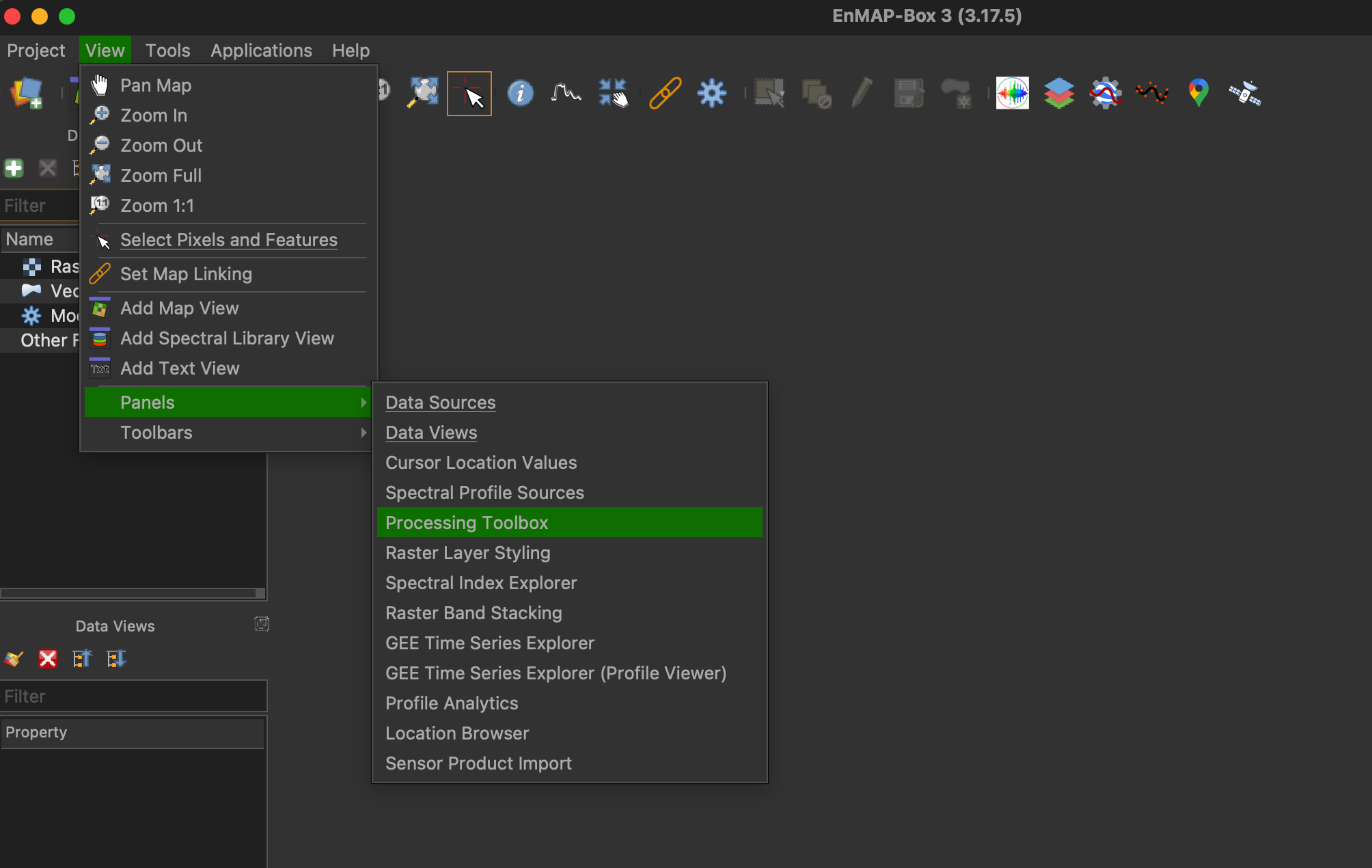
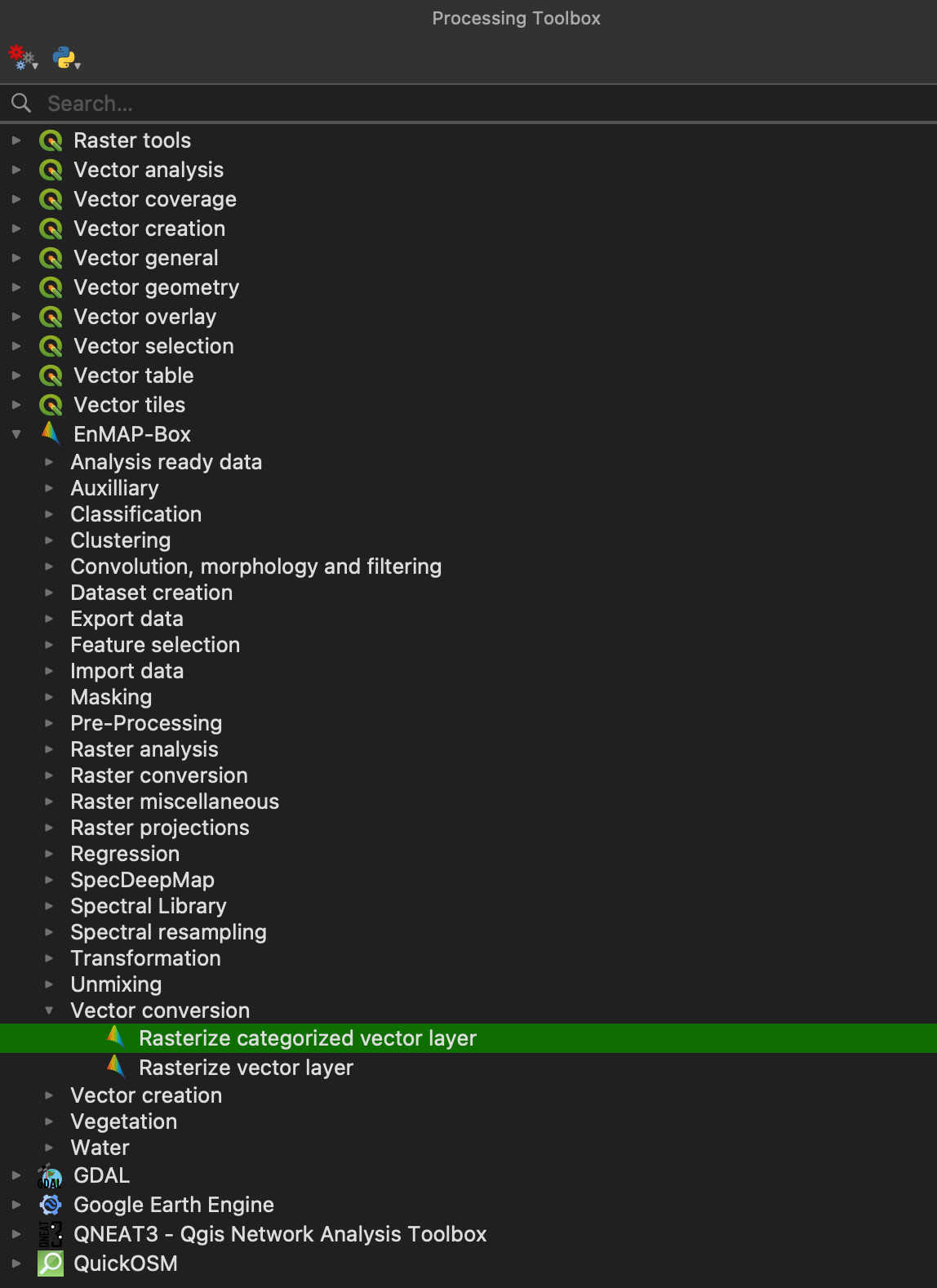
First of all, make sure the Processing Toolbox window is opened. If not, activate it via
View ‣ Panels ‣ Processing Toolbox
Open the Rasterize categorized vector layer algorithm under EnMAP-Box ‣ Vector conversion
 icon
in the QGIS toolbar or via from the menubar.
Furthermore, the EnMAP-Box Processing Algorithms provider is available in the Processing Toolbox.
icon
in the QGIS toolbar or via from the menubar.
Furthermore, the EnMAP-Box Processing Algorithms provider is available in the Processing Toolbox.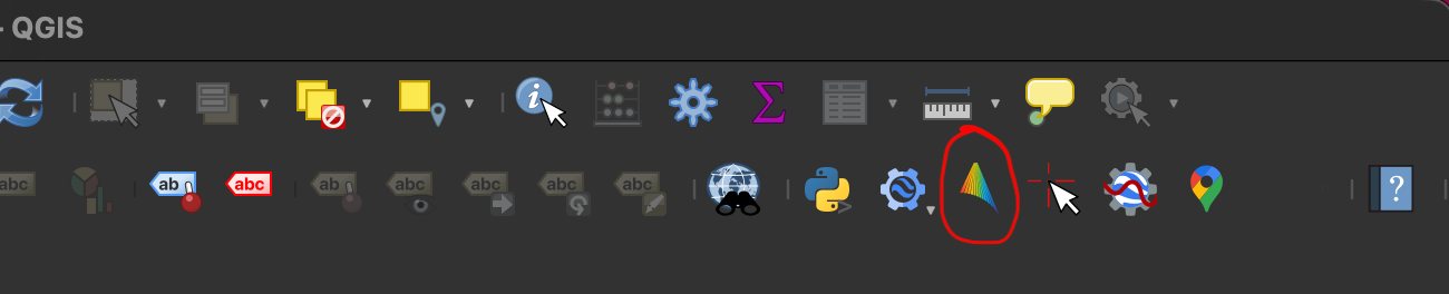
 Open a map view button to add a second map view. This view will appear below the
first map view (Map #1).
Open a map view button to add a second map view. This view will appear below the
first map view (Map #1).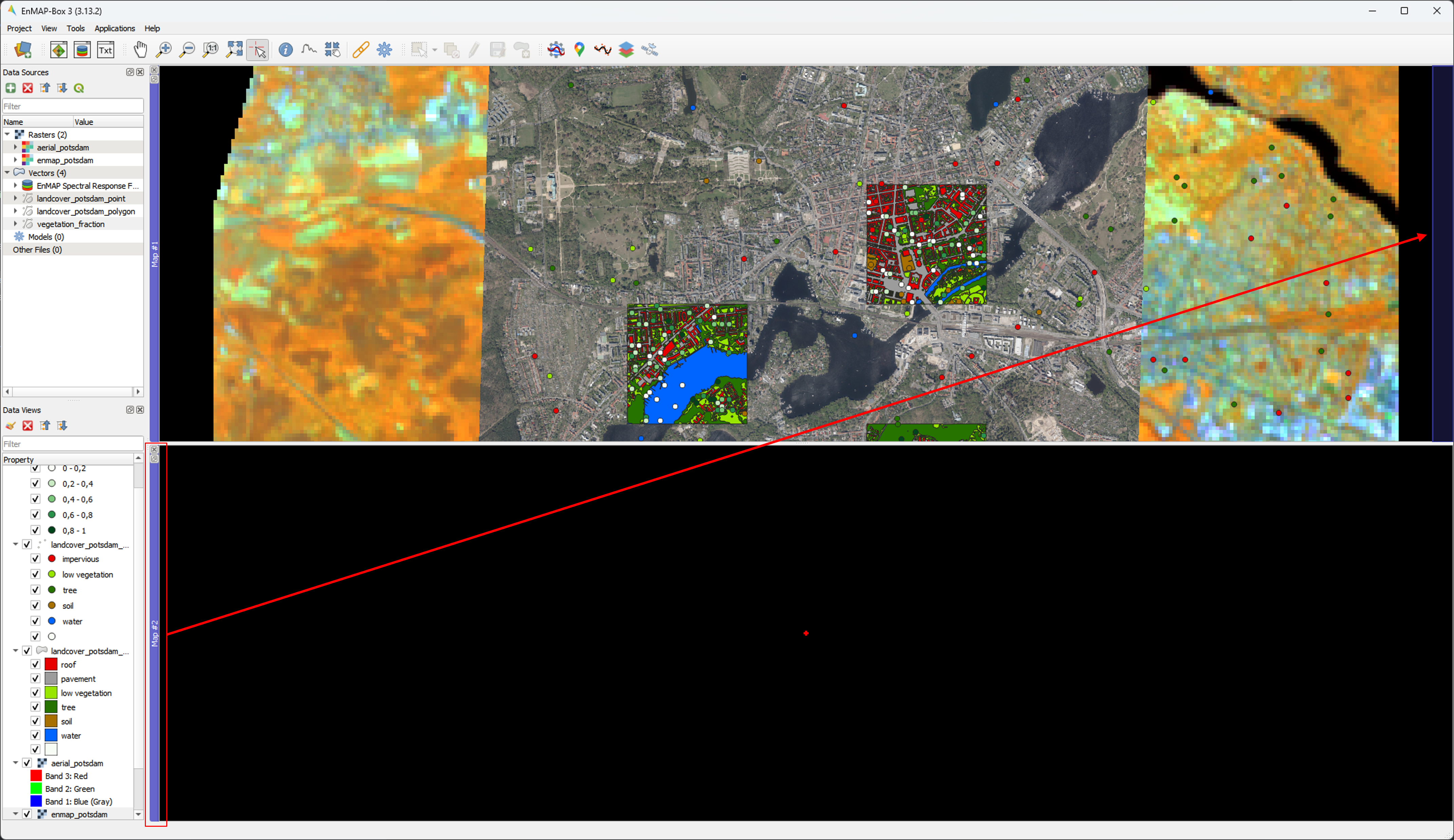
 button or go to and select
 Link map scale and center.
 or holding the mouse wheel
  ) and notice how both map views are synchronized now.
 Open Raster Layer Styling button, which will open
a new panel. Here you can quickly change the renderer (e.g., singleband gray, RGB) and the band(s) visualized. You can
do so manually using the slider or by selecting the buttons with predefined wavelength regions based on Sentinel-2 (e.g.
G = Green, N = Near infrared).
The raster layer needs to have wavelength information for the latter to work!
Open Raster Layer Styling button, which will open
a new panel. Here you can quickly change the renderer (e.g., singleband gray, RGB) and the band(s) visualized. You can
do so manually using the slider or by selecting the buttons with predefined wavelength regions based on Sentinel-2 (e.g.
G = Green, N = Near infrared).
The raster layer needs to have wavelength information for the latter to work! . You will find several band
combination presets. Select Colour infrared.
. You will find several band
combination presets. Select Colour infrared.
 on it) you can use the arrow keys ←/→ to
switch back and forth between bands!
on it) you can use the arrow keys ←/→ to
switch back and forth between bands!