Spectral Libraries

Spectral Libraries are collections of (i) spectral profiles and (ii) attributes that describe these profiles. The EnMAP-Box stores spectral profiles in vector layers. Compared to “traditional” spectral library formats like CSV text files or the ENVI Spectral library format, this has some advantages:

• We can link spectral profiles to geometries (points, lines, polygons) and easily display them in GIS maps. For example, the locations of measurements made with a field spectrometer.

• Spectral profiles can be linked with other spectral profiles. For example, a “target” measurement and the related “white reference” measurement can be stored together in the same vector layer feature.

• Spectral profiles can be linked with an arbitrary number of numeric, textual or categorical attributes, each having a dedicated data type. We can use QGIS/GDAL or data format-specific features to prevent incorrect values and ensure data integrity by design. For example, it can be ensured that leaf area index values have to be numeric and larger zero, or that values of an attribute material_type need to exist in a list of predefined material names.

• Spectral profiles can be stored in a wide range of data formats, ranging from local file types like GeoJSON or GeoPackage to powerful database management systems like PostgreSQL.. Each of them may have its own advantages, often specific to the project, user and metadata to be stored together with spectral profiles.

Since spectral profiles and their metadata are usually offered in different formats (ENVI, ASD, text files, …), the EnMAP-Box supports importing profiles from a wide range of file types.

Fig. 23 EnMAP-Box, showing profiles from the speclib_potsdam.zip example library, together with profiles collected from an EnMAP example image.

Spectral Library Viewer

The Spectral Library Viewer is the main tool to display spectral profiles in the EnMAP-Box. It shows profiles that can be stored in different Profile Fields and in different vector layers.

The plot settings panel on the right of the viewer is shown by activating the button. The panel is used to set up one or multiple profile visualizations. Each defines:

• The vector layer and Profile Fields to read the spectral profiles

• The profile styling: line type, symbol type, color. The color can be set statically or using a QGIS expression.

• The profile name: a QGIS expression that generates the name that is used in the legend

• An optional filter, for example to display only profiles matching a criterion like class_type=’vegetation’

The General Settings node allows to adjust the general appearance of the plot, e.g. by changing the background and foreground color, or activating the legend.

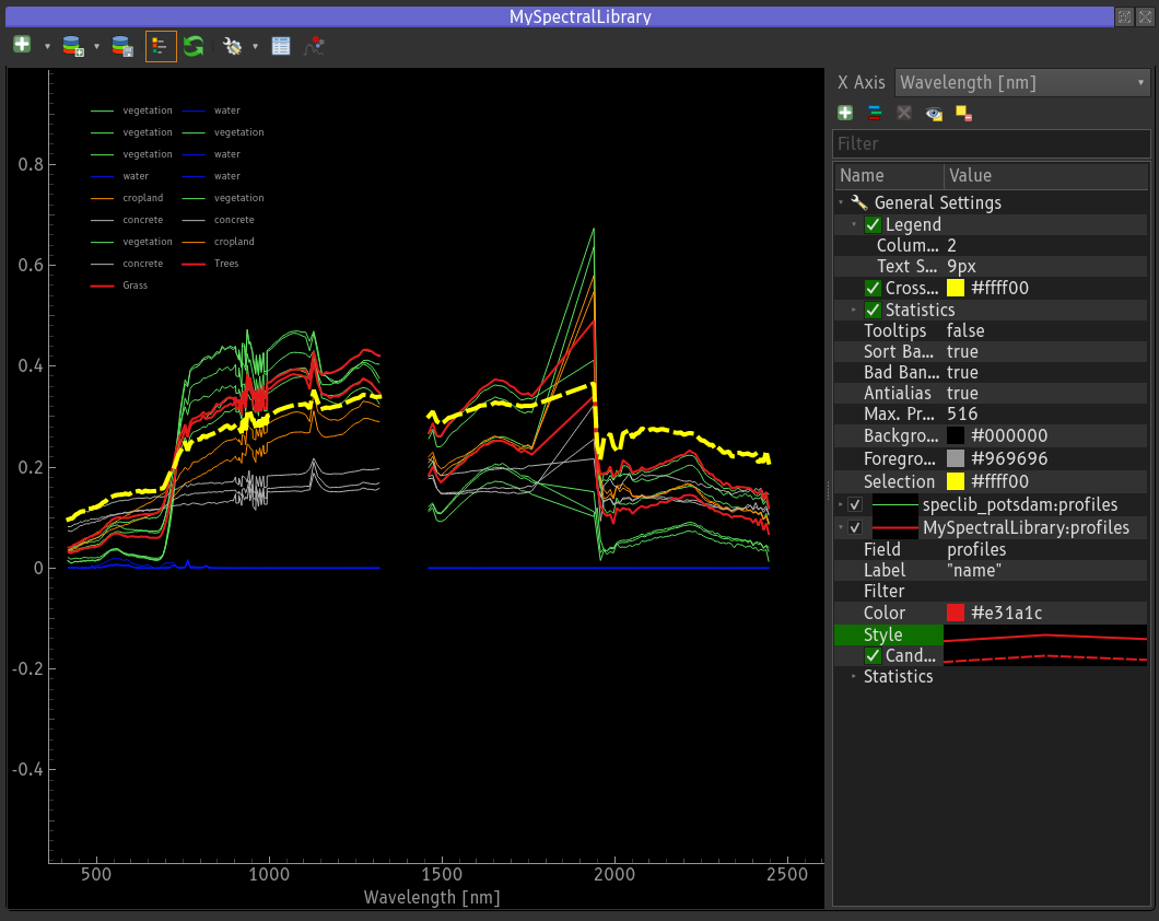
Fig. 24 Spectral Library Viewer

Selecting profiles in the profile plot does select the vector features the profile data is stored in. Selecting vector features in a map or attribute table does highlight the related profiles in the profile plot.

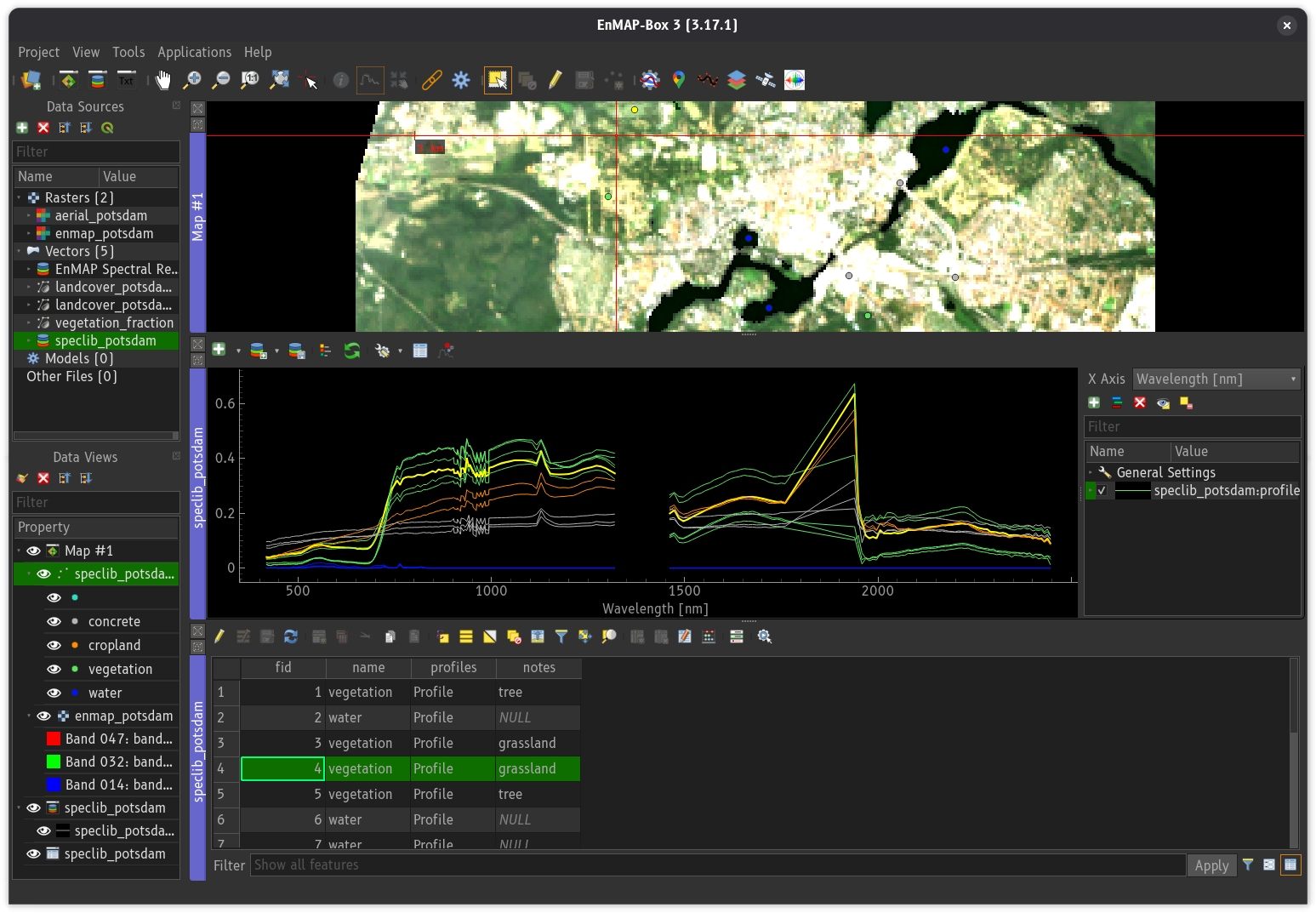
Fig. 25 When profiles are selected in the spectral library viewer, the corresponding vector features will also be selected in the map (top) and attribute table (bottom).

Attribute Table

The Attribute Table widget can be used to inspect and modify profile attributes. It displays vector data either in table view or using the form view . The form view for Spectral Profile fields allows to show spectral profile values as graph, JSON document or in a table.

Table View Form View

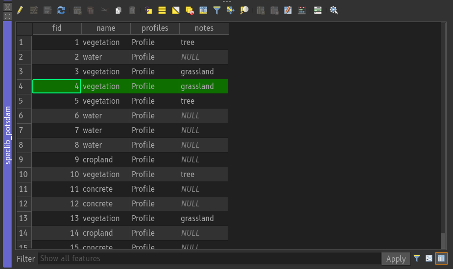
Fig. 26 Attribute table widget, showing spectral library attributes in table view.

The attribute table widget can be opened from different places, e.g., the context menu of a vector data source in the data sources panel or a vector layer in the layer tree of the data view panel.

In the Spectral Library Viewer it can be selected from the toolbar and the context menu of a profile visualization node, whose vector layer will then be opened in the attribute table widget.

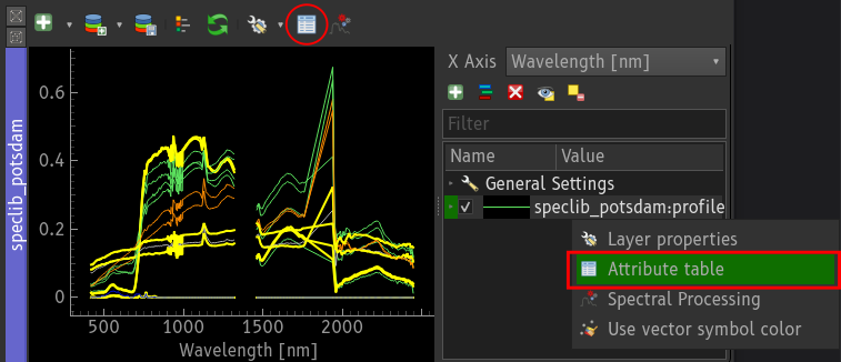
Fig. 28 Opening the attribute table for a vector layer whose profiles are shown in the spectral library viewer.

Profile Data

A single spectral profile contains the minimum information that is required to draw a profile. This information is stored in a JSON dictionary that contains at least a list y with profile values:

{
    "y": [0.1011, 0.1018, ... , 0.1080]
}

In addition it is possible to specify:

• x a list of position values along the x-axis, e.g. the band wavelength

• xUnit a string describing the unit of the x values

• yUnit a string describing the unit of the y values

• bbl a list of bad band multiplier values

If defined, the lists for x and bbl need to have the same length as y. Values in xUnit should use SI symbols wherever possible, e.g., μm instead of um or micrometers.

{
    "y": [0.1011, 0.1018, ... , 0.1080],
    "x": [418.24, 423.874, ... , 2445.53],
    "xUnit" : "nm",
    "yUnit" : "reflectance",
    "bbl" : [1, 0, ... , 1]
}

Modify spectral profiles

The EnMAP-Box is highly generic in how it supports raster and spectral data. After collecting spectral profiles, e.g. from raster images, by importing them from field measurements or sources like the USGS Spectral Library, the EnMAP Box offers different ways to modify them.

Profile Editor

Using the attribute table widget, the Form View for Spectral Profile fields can be used to edit profile values, either using a JSON editor or a table that lists the profile values.

1. Open the attribute table of a spectral library

2. Activate the form view

3. Activate the layer edit mode

4. Select the JSON or Table view

5. Edit the profile values

Fig. 29 Setting an outlier value to NaN.

Field Calculator

Simple calculations can be done using the QGIS Field Calculator.

1. Open an attribute table

2. Open the Field Calculator

3. Set a new field name or the name of a field you would like to update

4. Use the spectral_math function to calculate new profiles using a Python expression. Ensure that the output type meets the field type.

5. If a new field was created, use the layer settings to ensure that the editor widget type is set to Spectral Profile

Example: Calculate reflectance profiles

Let’s assume we have imported radiance measurements made with an ASD Field Spectrometer (for example, the *.asd files available here).

For each measurement we have the radiance profile of the white reference panel (reference) and the target surface (target). To obtain the surface reflectance, we need to divide the target radiance by the corresponding white reference radiance (https://eol.pages.cms.hu-berlin.de/geo_rs/S04_Lab_and_field_spectroscopy.html).

1. Open an attribute table

2. Open the Field Calculator

3. Define the output field. This can be a new field or an existing one.

4. Use the spectral_math function to calculate new profiles

   • define the input profiles. E.g., let p1 be the field with the reference radiance profiles and p2 the field with target radiance profiles.

   • define a Python expression that calculates output profiles. For example: y = y2 / y1 to divide target radiance by the reference radiance and obtain a reflectance profile.

   • ensure that the spectral_math function’s output type meets the type of the output field. For example, use format='text' if profiles are written into a string/varchar field.

5. Press ‘OK’

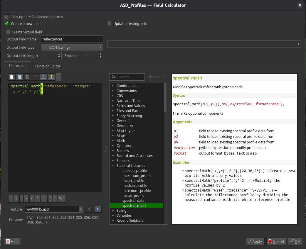
Fig. 30 QGIS field calculator with spectral_math function to calculate profile reflectances.

The spectral_math function makes input profile data available to the Python expression as follows:

• y -> y<n>, 1D numpy array, e.g., y1 for y values of the first input profile

• x -> x<n>, 1D numpy array, e.g., x1 for x values of the first input profile

• xUnit -> xUnit<n>, string, e.g., xUnit1 for the xUnit string of the first input profile

The output profile is specified using the following variables and default values:

• y numpy array or list with y values, defaults to y1

• x numpy array or list with x values, defaults to x1

• xUnit string with x unit, e.g., nanometers, defaults to xUnit1

Fig. 31 Calculating profile reflectances using the QGIS Field Calculator.

Spectral Processing

The Spectral Processing tool uses QGIS Processing Algorithms to process spectral profiles.

1. Open an EnMAP-Box Spectral Library viewer

2. Within the plot settings tree, select a profile source you would like to process.

3. Click the Spectral Processing button to open the Spectral Processing Dialog.

4. Select a processing algorithm that uses raster layers as input

5. Set your processing parameters.

6. Define the processing output. File names will be mapped into existing or new vector layer fields.

7. Click Run to start the processing.

Fig. 32 Using the Spectral Processing dialog to resample EnMAP profiles to Landsat.

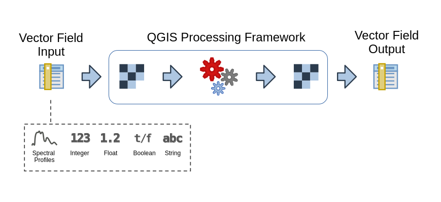
Fig. 33 The data flow handled by the Spectral Processing Dialog to use vector attribute values as raster inputs for QGIS Processing algorithms.

The Spectral Processing Dialog maps the attributes of a spectral library vector layer to temporary raster files. These files are then used as input for QGIS Processing Algorithms. Created raster outputs are converted back into attribute values for the spectral library vector layer. For example, the attribute fields of a spectral library with n = 20 features (aka rows in the Table view) are converted into rasters with one line and 20 pixels. The data type and number of bands of these temporary raster files depend on the input vector attributes.

Table 1 Mapping of vector attributes field values to temporary raster files

Field Type	Raster File
Spectral Profile	float raster with n > 1 bands
int / float	int / float raster with n = 1 band
string / any other data type	int classification image with n = 1 band. <br> Each unique string value is an individual class value

Table 2 Mapping of raster outputs into vector layer attributes

Raster File	Vector Field
n > 1 bands	Spectral profile
n = 1 band, int / float	int / float
n = 1 band, classification	string field containing the class name of each input pixel

Python Code

QGIS APIGDAL only

Todo

Add example

Profile Fields

The EnMAP-Box can read and write profile data into any vector layer field of the following data types:

Table 3 Datatypes to store spectral profiles

Data Type	SQL	GDAL/OGR	Qt/QGIS	Notes
Text, Strings	TEXT, VARCHAR			needs to support an arbitrary length
JavaScript Object Notation	JSON, JSONB		QVariantMap
Binary Large Objects	BLOB		QByteArray	deprecated, please use TEXT, VARCHAR or JSON data types

However, many text, JSON, and BLOB fields may be used for different purposes. It is therefore required to flag those fields that are used to store spectral profiles by setting the field’s editor widget type to SpectralProfile. This can be done in the Layer Property Dialog or via Python.

A *.qml sidecar file, e.g., myspeclib.qml next to myspeclib.gpkg, allows you to save layer properties like the editor widget type persistently. This way QGIS can restore them automatically when loading the vector source again.

Layer Property DialogPyQGISQML

To use a vector layer field for storing spectral profiles

1. Open the Layer Properties and select the Attributes Form page

2. Select the text or JSON field to store profiles

3. Choose SpectralProfile as Widget Type and Apply the changes

4. Call “Style” -> “Save as Default” to create a *.qml file that saves the layer style

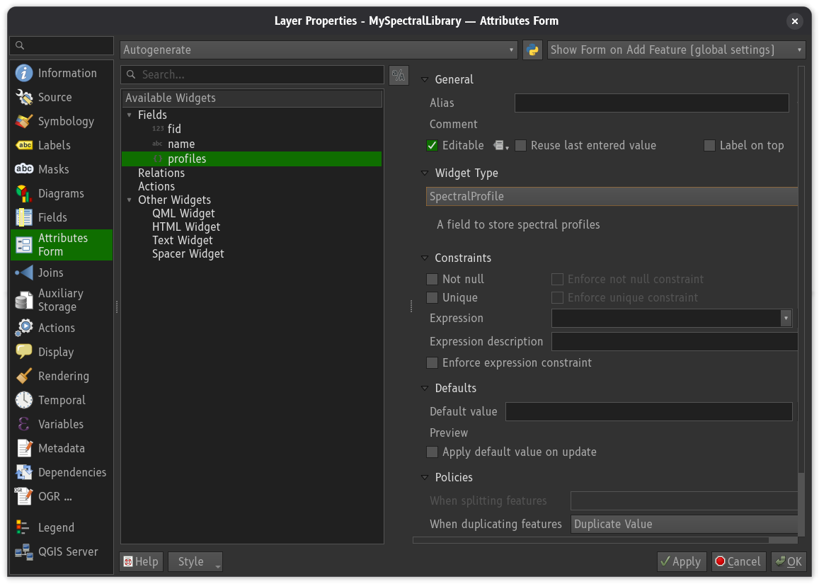
Fig. 34 The SpectralProfile widget type tells the EnMAP-Box, which layer fields can contain vector spectral profiles.

The profile fields of vector layers that are opened in the EnMAP-Box, e.g., as a layer in a map, can be selected as a source for a profile visualization

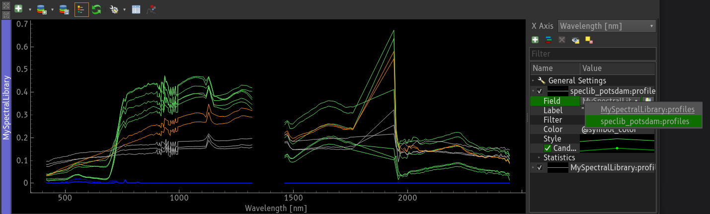
Fig. 35 Selection of a profile field as a source for a visualization.

Collect Profiles

To collect spectral profiles from raster layers, go into the toolbar and activate the Identify map tool with option Identify pixel profiles .

Now click on a raster pixel. By default, this creates a new in-memory vector layer “Profiles #1” and opens a spectral library view to show it. The Spectral Profile Sources panel can be used to specify how profiles are collected, e.g., from which raster layer, and to which vector layer field they will be written. In addition, it allows you to specify values for other fields of the vector layer, e.g., to generate a profile name automatically.

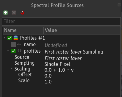
Fig. 36 The spectral profile source panel describes how profiles are collected and written to vector layers.

Import Profiles

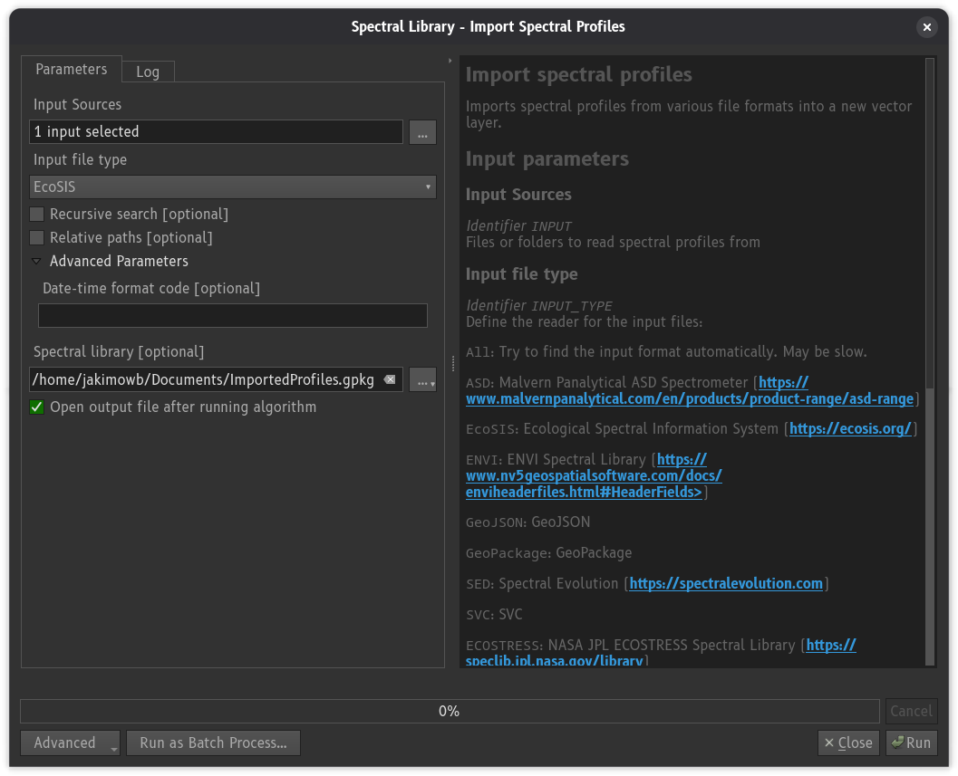
The Import Spectral Profiles algorithm loads profiles from different sources into a new vector layer. It can be opened from the Spectral Library Viewer, using the button, or from the QGIS processing toolbox (enmapbox:importspectralprofiles).

The import algorithm tries to identify the format of each source file on its own. However, to improve speed it is recommended to specify the file input type manually.

Table 4 File types from which spectral profiles can be imported

Input File Type	Description
ASD	Binary file output created by ASD Field Spectrometers
ECOSTRESS	CSV text files from the NASA JPL ECOSTRESS Spectral Library https://speclib.jpl.nasa.gov/
ENVI	ENVI Spectral Library binary format
EcoSIS	CSV text files from the Ecological Spectral Information System (EcoSIS)
GeoJSON	EnMAP-Box Spectral Library, saved as GeoJSON
GeoPackage	EnMAP-box Spectral Library, saved as GeoPackage
SED	Text file output created by Spectral Evolution Spectroradiometers
SVC	Text file output created by Spectral Vista Corporation Spectroradiometers

Export Profiles

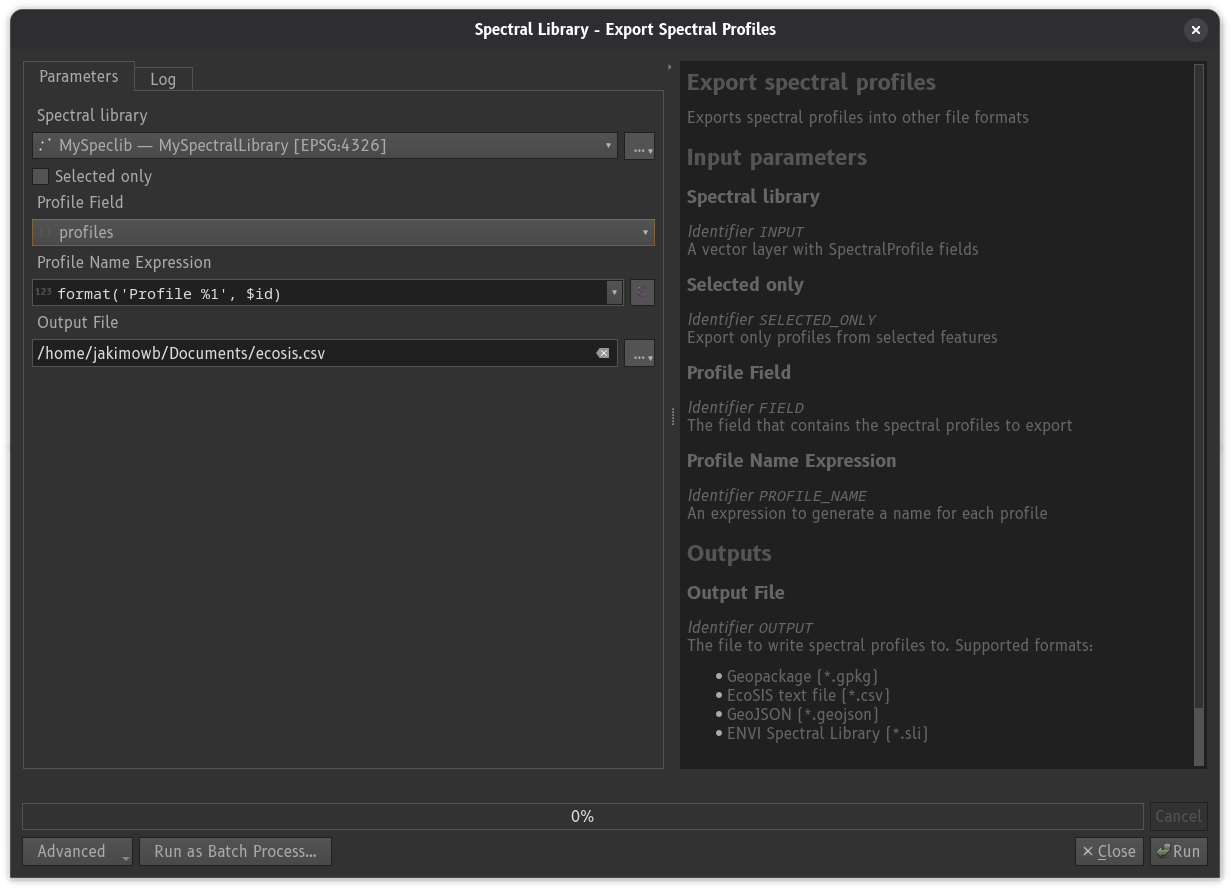
The Export Spectral Profiles algorithm allows to save spectral profiles in other file formats. It can be opened either from the Spectral Library Viewer, using the button, or from the QGIS processing toolbox (enmapbox:exportspectralprofiles).

The algorithm requires to specify the Profile Field whose profiles are to be saved, and a field or QGIS expression to get a profile name from.

Table 5 File types into which spectral profiles can be exported

Export File Type	Extension	Description
ENVI Spectral Library	*.sli	ENVI Spectral Library binary format
EcoSIS	*.csv	CSV text files used by Ecological Spectral Information System (EcoSIS)
GeoJSON	EnMAP-Box Spectral Library, saved as GeoJSON
GeoPackage	EnMAP-box Spectral Library, saved as GeoPackage