Earth Observation for QGIS (EO4Q)
Earth Observation for QGIS (EO4Q) is a collection of EnMAP-Box tools and applications designed to integrate well in both, EnMAP-Box and QGIS environments. In both environments, EO4Q applications can be started from the Earth Observation for QGIS (EO4Q) Toolbar:
GEE Time Series Explorer
The GEE Time Series Exlorer integrates Google Earth Engine (GEE) into QGIS/EnMAP-Box. It allows the interactive exploration of temporal raster data available in the Earth Engine Data Catalog .
A first version of the GEE Time Series Exlorer was released as a QGIS plugin. Future versions will be maintained as an EO4Q application that integrates into QGIS and EnMAP-Box GUI.
Live demonstration
- Slides from the Living Planet Symposium 2022 talk in Bonn, Germany
Janz, A. et al. (2022, May 26). GEE Time Series Explorer: Planetary-scale visualization and temporal profile sampling of EO imagery from the Earth Engine Data Catalog in QGIS and the EnMAP-Box [oral presentation]. Living Planet Symposium, Bonn, Germany
- How to cite
Rufin, P., Rabe, A., Nill, L., and Hostert, P. (2021) GEE TIMESERIES EXPLORER FOR QGIS - INSTANT ACCESS TO PETABYTES OF EARTH OBSERVATION DATA , Int. Arch. Photogramm. Remote Sens. Spatial Inf. Sci., XLVI-4/W2-2021, 155-158, https://doi.org/10.5194/isprs-archives-XLVI-4-W2-2021-155-2021, 2021.
- Used in scientific research
Marionei Fomaca de Sousa Junior, Leila Maria Garcia Fonseca and Hugo do Nascimento Bendini (2022) Estimation of Water Use in Center Pivot Irrigation Using Evapotranspiration Time Series Derived by Landsat: A Study Case in a Southeastern Region of the Brazilian Savanna
Philippe Rufin, Mayra Daniela Peña-Guerrero, Atabek Umirbekov, Yanbing Wei and Daniel Müller (2022) Post-Soviet changes in cropping practices in the irrigated drylands of the Aral Sea basin
Philippe Rufin, Adia Bey, Michelle Picoli, Patrick Meyfroidt (2022) Large-area mapping of active cropland and short-term fallows in smallholder landscapes using PlanetScope data
Agência Nacional de Águas. Atlas Irrigação: Uso Da Água Na Agricultura Irrigada , 2nd ed.; Agência Nacional de Águas: Brasilia, Brazil (2021)
- Prerequisite
The GEE Time Series Exlorer depends on the QGIS Google Earth Engine plugin . In order to access Earth Engine, you must have an Google account that is authorized for Earth Engine. If you haven’t used Earth Engine so far, the easiest way to make sure that everything is working on your system, is to follow the instruction here: https://gee-community.github.io/qgis-earthengine-plugin/
Getting started
- Usage
Start the application from the View > Panels > GEE Time Series Exlorer menu or from the Earth Observation for QGIS (EO4Q) Toolbar
 .
.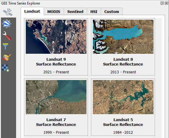
Fig. 46 GEE Time Series Explorer main panel, showing the Data Catalog tab with Landsat collections.
Select a collection.
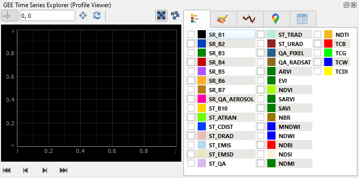
Fig. 47 GEE Time Series Explorer (Profile Viewer) panel, showing available bands and spectral indices.
- Load a collection, plot a temporal profile and visualize an image
Select the Landsat 8 Surface Reflectance collection in the Data Catalog tab of the main panel.
Select the NDVI band in the Profile Viewer panel.
Activate the Current Location map tool
 and select a location on the map.
This will plot the temporal profile for that location in the Profile Viewer panel.
and select a location on the map.
This will plot the temporal profile for that location in the Profile Viewer panel.Select a data point in the plot to visualize the associated image. The image is displayed in it’s default visualization.
- Improve image contrast stretch
The default visualization may give a poor image contrast, which you may want to improve. In the Band Rendering tab of the main panel, you may set suitable min/max values manually, or specify lower/upper percentile cut off values, e.g. 2% to 98%. Note that the statistics are calculated for the current map extent.
- Visualize derived vegetation indices
Beside visualizing original image bands in Multiband color RGB, it is possible to visualize derived vegetation indices.
- Prepare a cloud-free composite
To create a composite that aggregates all images in a given date range, we just switch from Image Selection mode to Composite Selection mode in the Profile Viewer panel. In the plot we can now select a date range and create our first, very cloudy, composite. By applying a Pixel Quality Filter we can easily exclude all pixel affected by cloud and cloud shadow. And finally, we can improve the contrast stretch of the visualization.
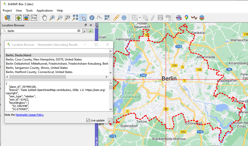
Location Browser
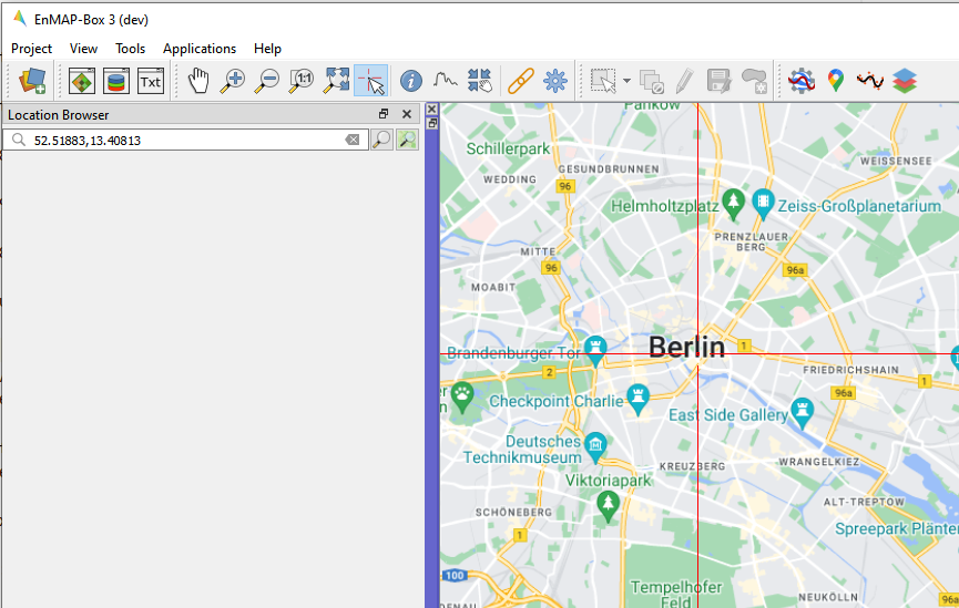
The Location Browser panel allows to a) navigate to a map location directly, or to b) send a request to the Nominatim geocoding service.
- Usage
Start the tool from the View > Panels > Location Browser menu or from the Earth Observation for QGIS (EO4Q) Toolbar.
Go to locations directly by entering the coordinates in one of the following formats:
53.07478793449, 13.895089018465338(longitude, latitude in decimal format)53°04'29.2"N, 13°53'42.3"E(longitude, latitude in GPS format)13.895089018465338, 53.07478793449, [EPSG:4326](east, north, EPSG ID)
Or send a request to the Nominatim geocoding service and explore the results:
berlin(free-form textual description of the location to be geocoded)
- GUI
- Live demonstration
Profile Analytics
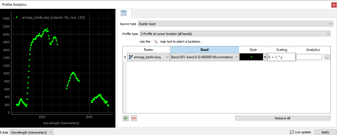
The Profile Analytics panel allows to visualize various types of spectral, temporal and spatial profiles. Additionally, profile data can be analysed by user-defined functions (ufuncs). A ufunc has access to the plot widget and can draw additional plot items.
- Usage
Start the tool from the View > Panels > Profile Analytics menu or from the Earth Observation for QGIS (EO4Q) Toolbar.
Select the Source type, that is providing the profiles. Note that we’re currently only support raster layer as source, but we plan to have other sources like profiles from the GEE Time Series Explorer.
Select the Profile type you want to extract from the raster layer:
Select a Raster.
In case of a spatial profile (i.e. X-Profile, Y-Profile and Profile along a line), also select a Band. In case of a Z-Profile), the selected band is ignored.
Style the profile.
Apply data Scaling.
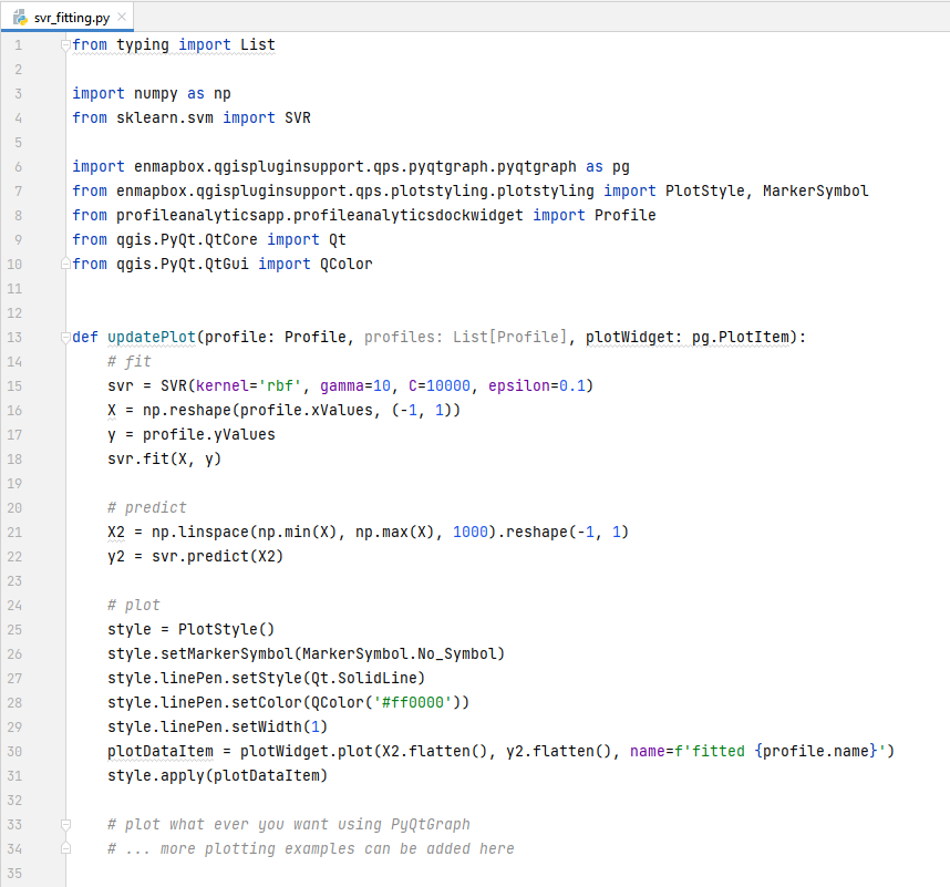
Choose an ufunc to perform Analytics on the profile data and add extra plot annotations. The ufunc has full access to the plot widget and can add plot items like:
plot line (e.g. fitted data, vegetation regrowth, trend lines, etc.)
plot marker symbols (e.g. forest clear cut events, mowing events, fire events, red-edge inflection point, etc.)
plot text
insert images
Examples can be found under
/enmapbox/eo4qapps/profileanalyticsapp/examples/.Depending on the Profile type and availability of raster metadata, different X Axis units can be choosen:
Z-Profile values:
can always be plotted against Band Numbers
can be plotted against Wavelength, if band center wavelength is specified
can be plotted against Date Time, if band (aquisition) date time is specified
X-Profile values are always plotted against the Column Number.
Y-Profile values are always plotted against the Row Number.
Profile along a line values are always plotted against the Distance from line start.
In case of X-Profile, Y-Profile and Z-Profile, use the Cursor Location map tool to select a location that specifies the profile.
In case of Profile along a line, use the Select Feature map tool to select a line-vector feature that specifies the profile.
- GUI
- Spectral Z-Profile
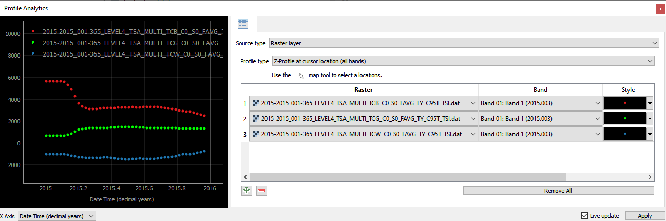
- Temporal Z-Profiles
- Temporal Z-Profile annotated with a Support Vector Regression fit (
svr_fitting.pyused as ufunc) 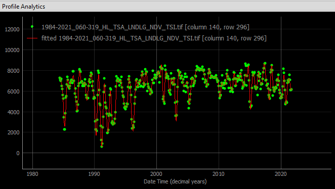
- Live demonstration
Raster Band Stacking
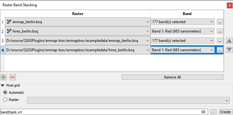
The Raster Band Stacking panel allows to stack bands into a new VRT raster layer. Raster bands can be selected inside the panel or added via drag&drop in various ways.
- Usage
Start the tool from the View > Panels > Raster Band Stacking menu or from the Earth Observation for QGIS (EO4Q) Toolbar.
Add raster sources and select bands:
add a new raster source via the “+” button
select raster(s) inside the Data Sources panel and drag&drop the selection into the table
select band(s) inside the Data Sources panel and drag&drop the selection into the table
select raster layer(s) inside the Data Views panel and drag&drop the selection into the table
select raster files inside the file explorer (e.g. Windows Explorer) and drag&drop the selection into the table
Prepare the final band stack inside the table by:
changing individual band selections
removing rows
moving rows up and down
Choose an output filename and create the band stack. By default, the output pixel grid (i.e. extent, resolution, crs) is derived automatically (i.e. gdal.BuildVrt defaults). To use a custom pixel grid, switch to the Raster option and select a raster.
- GUI
- Live demonstration
Sensor Product Import
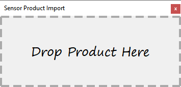
The Sensor Product Import panel allows to import various sensor products via drag&drop. E.g. a downloaded Landsat product can be imported as is:
- Landsat 9 Product Example
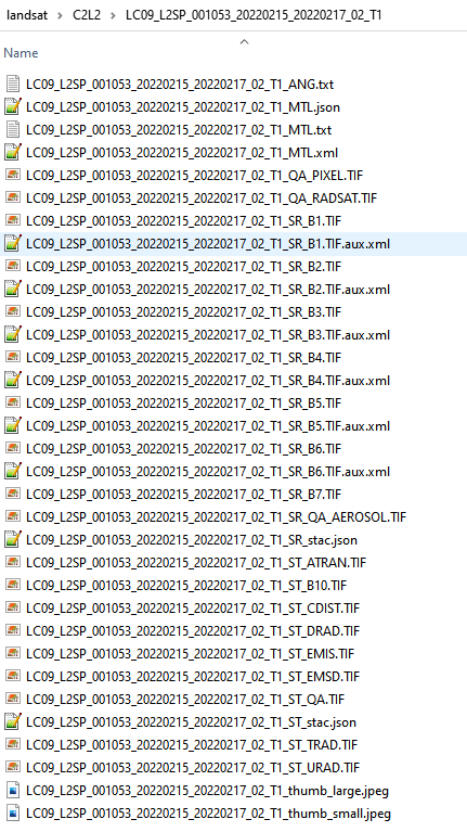
All the surface reflectance bands are automatically stacked, band offset and scaling factors are applied, and proper metadata, like center wavelength and band names, are specified.
- Usage
Start the tool from the View > Panels > Sensor Product Import menu or from the Earth Observation for QGIS (EO4Q) Toolbar.
Drag&drop the product folder, or any file inside the product folder, into the Drop Product Here area.
Run the import algorithm. Note that the result is stored next to the source product. When opening the product for the next time, this algorithm is not shown.
Visualize the result raster.
- GUI
Live demonstration
Spectral Index Explorer
The Spectral Index Explorer panel allows to derive spectral indices for a spectral raster. Indices can be selected from the ready-to-use curated list of Awesome Spectral Indices for Remote Sensing applications, maintained by David Montero Loaiza.
- Usage
Start the tool from the View > Panels > Spectral Index Explorer menu or from the Earth Observation for QGIS (EO4Q) Toolbar.
Select a Source layer, e.g. a multi- or hyperspectral raster.
[Optional] Check the Band Identifiers table to make sure that common wavebands are correctly matched with source raster layer bands. Feel free to correct the default matching, which is derived from wavelength metadata.
[Optional] Check the Constants table to make sure that constants are properly defined. Feel free to change default values.
Select a spectral index from the Spectral Indices table to create a new spectral index layer.
b) Alternatively, choose Layer name and Formula manually to create a custom spectral index.
- GUI

- Live demonstration