Applications

Agricultural Applications

Please visit LMU Vegetation Apps Documentation for more information.

Classification Dataset Manager

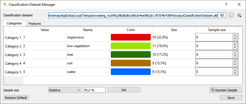
The Classification Dataset Manager allows to a) create a new dataset from various sources, b) presents basic information for each category like value, name, color and number of samples, c) supports editing of category names and colors, and d) let’s you easily draw a random sample.

Usage

1. Start the tool from the Applications > Classification Dataset Manager menu.

2. Use the tool for different cases like:

   • create a dataset

   • edit a dataset

   • draw a random subsample

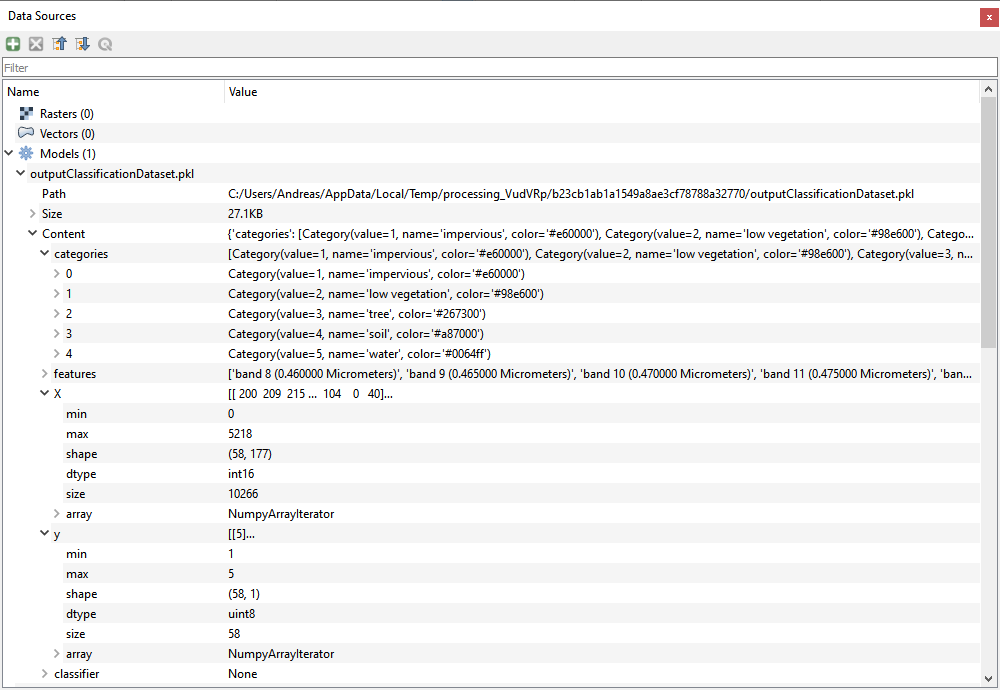
3. Inspect created datasets inside the Data Sources panel.

GUI

Live demonstration

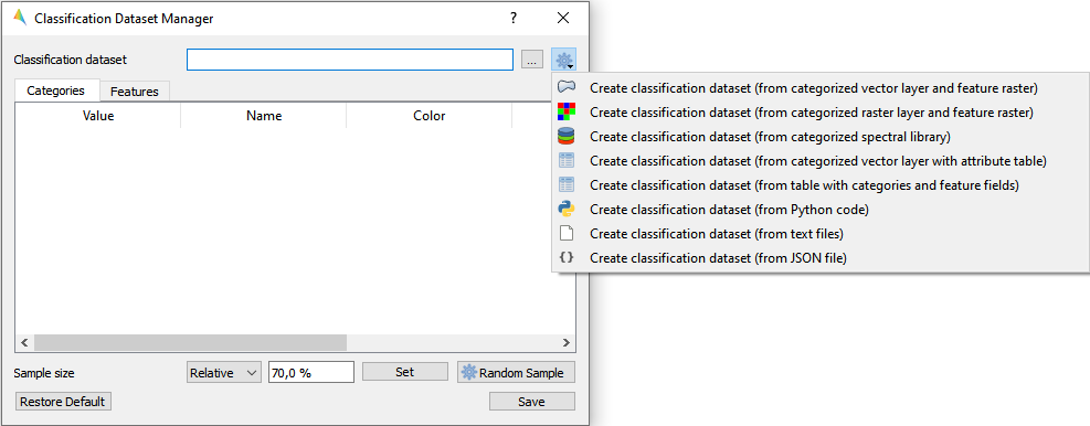
Create a classification dataset

Select one of the dataset creation options and follow the subsequent algorithm dialog.

GUI

Example data

Datasets used below are available in of the following locations:

• enmap-box/enmapbox/exampledata/

• enmap-box/tests/testdata/

From categorized vector layer and feature raster

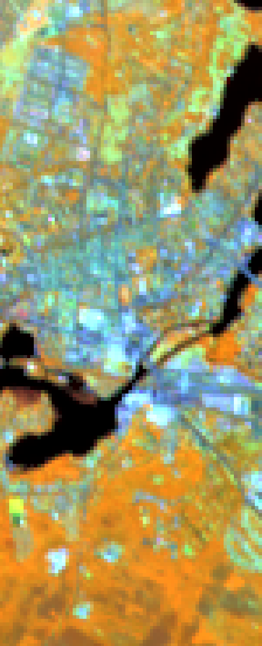
Fig. 15 enmap_potsdam.bsq

Fig. 16 landcover_potsdam_point.gpkg

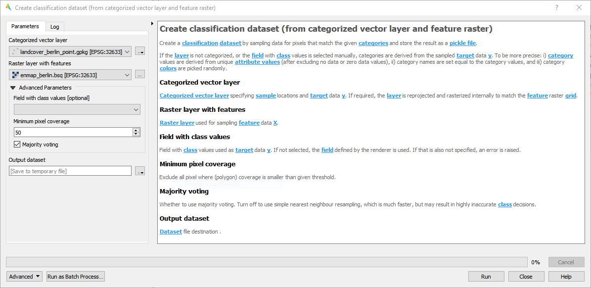
For details see the algorithm description.

From categorized raster layer and feature raster

Fig. 17 enmap_potsdam.bsq

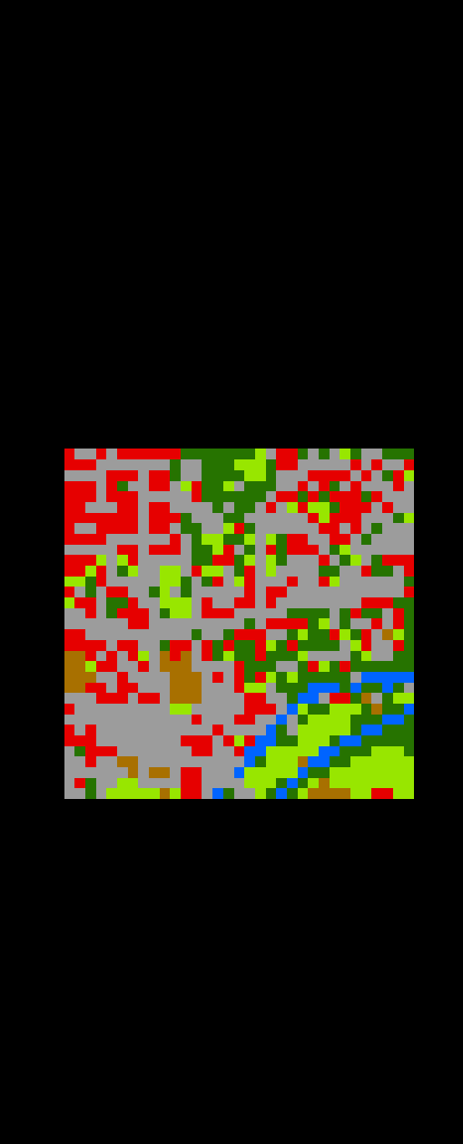
Fig. 18 landcover_polygon_30m.tif

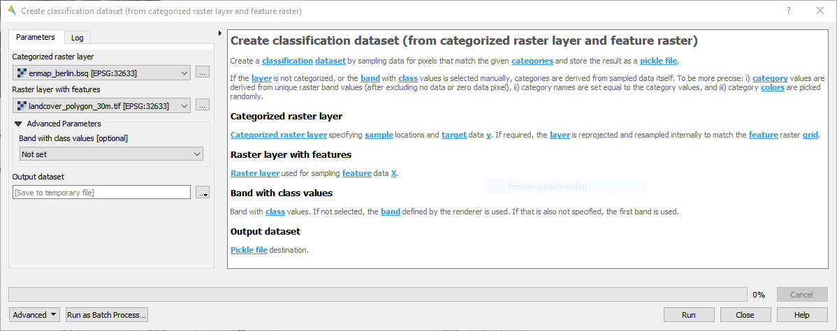
For details see the algorithm description.

From categorized spectral library

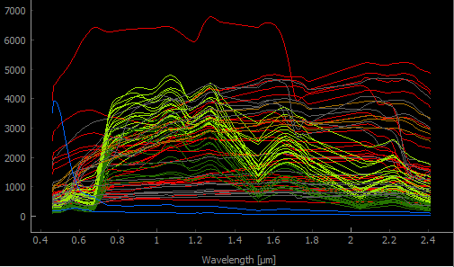
Fig. 19 library_potsdam.gpkg

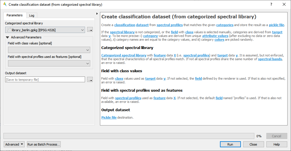
For details see the algorithm description.

From categorized vector layer with attribute table

Fig. 20 classification_dataset.gpkg

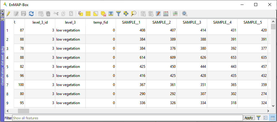
Fig. 21 Attribute table with fields Sample_1, Sample_2, … Sample_177 used as features.

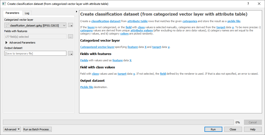
For details see the algorithm description.

From table with categories and feature fields

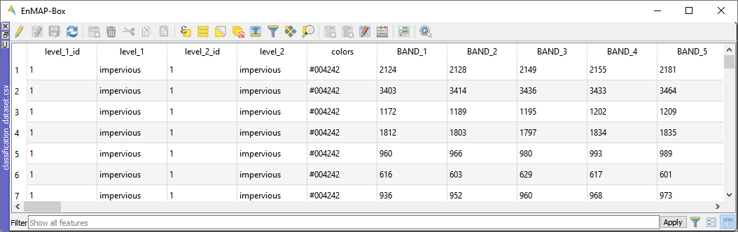
Fig. 22 Attribute table with fields Band_1, Band_2, … Band_177 used as features.

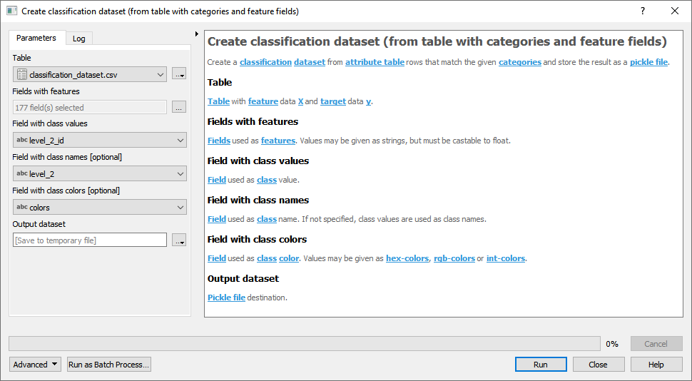
For details see the algorithm description.

From Python code

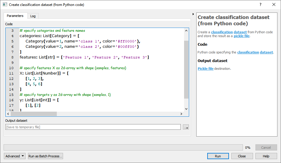
For details see the algorithm description.

From text files

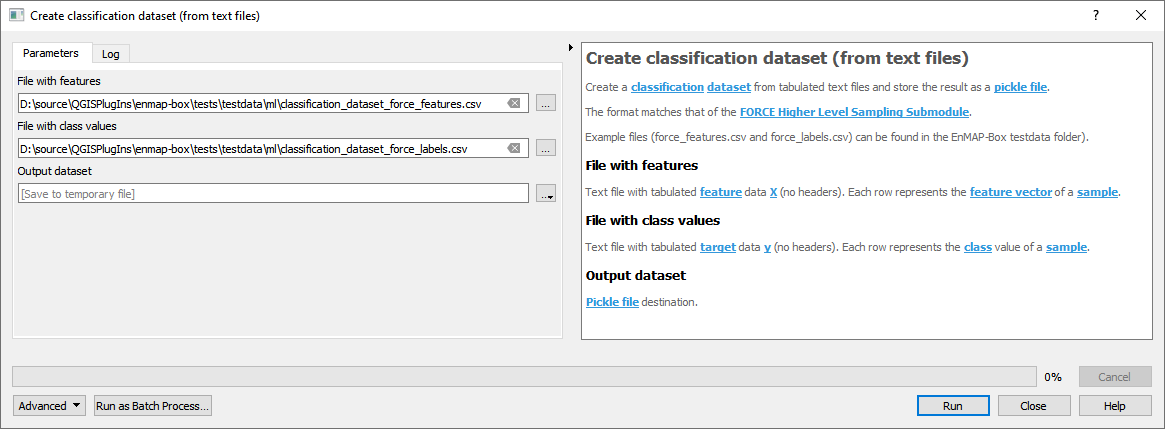
For details see the algorithm description.

From JSON file

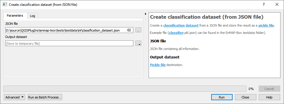
For details see the algorithm description.

Edit categories and features

Usage

1. Select a classification dataset.

2. Edit category names and colors inside the Categories tab.

3. Edit feature names inside the Features tab.

4. Save the edits.

Split dataset randomly

Usage

1. Select a classification dataset.

2. Set the sample size for each category to be drawn inside the Categories tab.

   Alternatively, Set a relative or absolute sample size used for all categories.

3. Click Random Sample and follow the subsequent algorithm dialog.

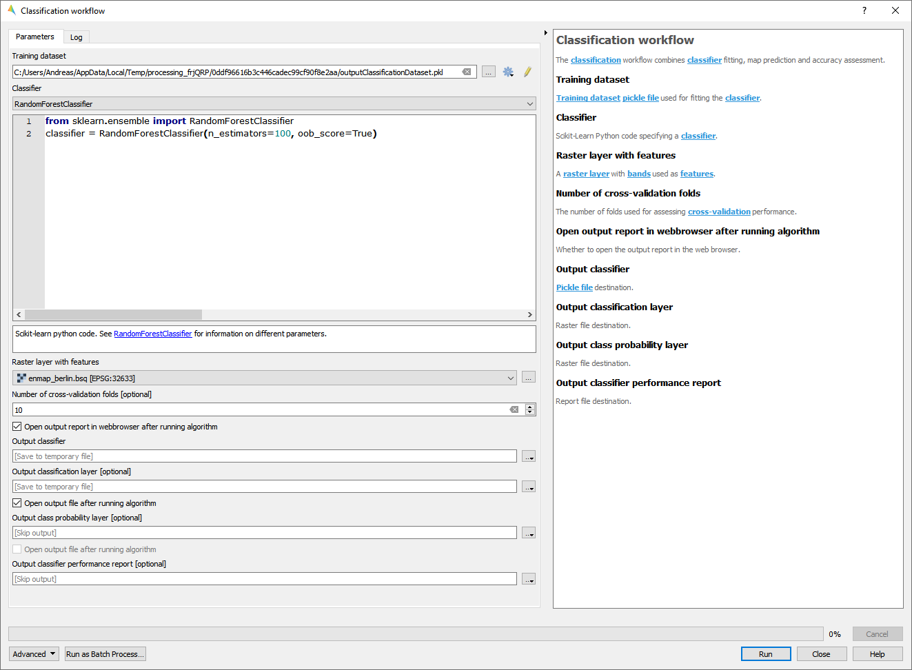
Classification workflow

The Classification workflow algorithm let’s you easily perform classification analysis and mapping tasks using remote sensing data.

Usage

1. Start the algorithm from the Applications > Classification workflow menu.

2. Select a Training dataset.

3. Select a Classifier.

4. Select a Raster layer with features used for mapping.

5. If cross-validation accuracy assessment is desired, select the Number of cross-validation folds and a Output classifier performance report file destination (this step is skipped by default).

6. If the classifier supports class probability, you may select an Output class probability layer file destination (this step is skipped by default).

7. Click Run.

GUI

Live demonstration

Classification Workflow (advanced)

The Classification Workflow application let’s you easily perform classification analysis and mapping tasks using remote sensing data.

Quick Mapping

In the Quick Mapping section you can very easily define your training dataset, fit a classifier and predict a classification layer, with only a few clicks.

Live demonstration

For a more elaborated analysis see the Detailed Analysis section.

Detailed Analysis

In the Detailed Analysis section you have more control over individual analysis steps. When performing a detailed analysis, you can basically go through every subsection from left to right. But, depending on the usecase, it is also possible to skip individual steps you’re not interested in.

Live demonstration

Dataset

You have various options to create a dataset for subsequent analysis: select a Source option and click create dataset to create a new dataset`.

In the Editor, category colors and names, and feature names can be changed and saved.

By using the various controls in the Draw samples section, you can easily define a training-test-split setup. The number of training and test samples to be drawn for each category are listed, and also editable, inside the Editor.

Click split dataset to perform the split, resulting in a training and a test dataset, that can be used in subsequent analysis.

Classifier

In the Classifier section you can either select a Predifined classifier or provide a user-defined Python Code snipped. See the https://scikit-learn.org/ documentation for a complete overview.

Click create classifier to create an (unfitted) classifier, that can be used in subsequent analysis.

Feature Clustering

In the Feature Clustering section you can perform an unsupervised Feature redundancy analysis, that clusters similar features together: select a Dataset, an Algorithm and click cluster features to create and an Output report.

After inspecting the report you can perform a Feature subset selection: select a suitable Number of features and click select features to create a training and a test dataset with fewer features, that are less correlated and can be used in subsequent analysis.

Feature Ranking

In the Feature Ranking section you can perform a supervised Feature importance analysis, that ranks features in terms of their importance for the classification task at hand: select a Dataset, an Algorithm and click :guilabel:`rank features to create and an Output report.

After inspecting the report you can perform a Feature subset selection: select a suitable Number of features and click select features to create a training and a test dataset with fewer features, that are most important and can be used in subsequent analysis.

Model

In the Model section you can perform Model fitting: select a Dataset and click fit classifier to create a fitted Output classifier, that is used in subsequent analysis.

For Model performance analysis select an Algorithm and click assess performance to create an Output report.

Classification

In the Classification section you can perform Map prediction: select a Raster layer with features that matches the features used in Model fitting. Click predict output products to create an Output classification layer and/or an Output class probability layer. Note that outputs are opened inside the EnMAP-Box Data Sources panel.

For Map accuracy and area estimation select a Ground truth categorized layer and click assess performance to create an Output report.

Settings

In the Settings section you can specify the Output directory (e.g. C:/Users/USERNAME/AppData/Local/Temp/EnMAPBox/ClassificationWorkflow), that is used as the default file destination path, when creating file outputs. Note that each output file wigdet (e.g. Output dataset) has a default basename (e.g. dataset.pkl), that is used to create a default file destination (e.g. C:/Users/USERNAME/AppData/Local/Temp/EnMAPBox/ClassificationWorkflow/dataset.pkl). If the default file destination already exists, the basename is enumerated (e.g. .dataset_2.pkl) to avoid overwriting existing outputs.

Log

Classification Workflow (deprecated)

Deprecated, use Classification workflow or Classification Workflow (advanced) instead.

You can find this application in the menu bar Applications ‣ Classification Workflow Classic

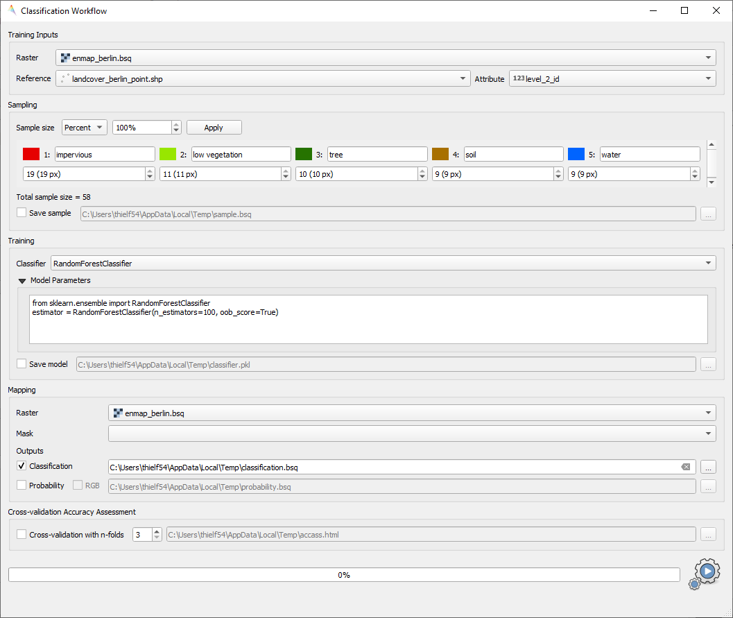
Fig. 23 Classification Workflow Application

See also

Have a look at the Getting Started for a use case example of the Classification Workflow Application.

Input Parameters:

• Training Inputs

  • Type

    Three different types of input data sources are supported and have to be specified beforehand in the dropdown menu. Depending on the selected input type the user interface shows different options.

    • Raster / Classification:

      • Raster: Specify input raster based on which samples will be drawn for training a classifier.

      • Classification: Specify input raster which holds class information.

    • Raster / Vector Classification:

      • Raster: Specify input raster based on which samples will be drawn for training a classifier.

      • Reference: Specify vector dataset with reference information. Has to have a column in the attribute table with a unique class identifier (numeric). The class colors and labels are derived from the current Symbology. To set or change those settings, click the button or go to the Layer Properties (Layer properties ‣ Symbology). The vector dataset is rasterized/burned on-the-fly onto the grid of the input raster in order to extract the sample. If the vector source is a polygon dataset, only polygons which cover more than 75% of a pixel in the target grid are rasterized.

    • labelled Library:

      • Library: Specify input spectral library.

• Sampling

  Once you specified all inputs in the Training inputs section, you can edit the class colors, names and class sample sizes in the Sampling submenu.

  Note

  If set, the class labels and color information is automatically retrieved from the layers current renderer settings (Layer properties ‣ Symbology).

  • Sample size Specify the sample size per class, either relative in percent or in absolute pixel counts.

  • The total sample size is shown below

  • Save sample: Activate this option and specify an output path to save the sample as a raster.

• Training

  • In the Classifier dropdown menu you can choose different classifiers (e.g. Random Forest, Support Vector Machine)

  • Model parameters: Specify the parameters of the selected classifier.

    Hint

    Scikit-learn python syntax is used here, which means you can specify model parameters accordingly. Have a look at the scikit-learn documentation on the individual parameters, e.g. for the RandomForestClassifier

  • Save model: Activate this option to save the model file (.pkl) to disk.

• Mapping

  • Raster: Specify the raster you would like to apply the trained classifier to (usually -but not necessarily- this is the same as used for training)

  • Mask: Specify a mask layer if you want to exclude certain areas from the prediction.

    • Outputs:

      • Classification: Output path where to write the classification image to.

      • Probability: Output path of the class probability image.

        Hint

        This outputs the result of a classifiers predict_proba method. Note that depending on the classifier this option might not be available or has to be activated in the model parameters (e.g. for the Support Vector Machine, the line svc = SVC(probability=False) has to be altered to svc = SVC(probability=True)

      • RGB: Generates a RGB visualisation based on the weighted sum of class colors and class probabilities.

• Cross-validation Accuracy Assessment

  • Cross-validation with n-folds : Activate this setting to assess the accuracy of the classification by performing cross validation. Specify the desired number of folds (default: 3). HTML report will be generated at the specified output path.

Run the classification workflow

Once all parameters are entered, press the button to start the classification workflow.

EO Time Series Viewer

Please visit EO Time Series Viewer Documentation for more information.

EnPT (EnMAP Processing Tool)

Please visit EnPT Tutorial for more information.

GFZ EnGeoMAP

Please visit EnGeoMAP Tutorial for more information.

Image Math (deprecated)

Deprecated, use Raster math

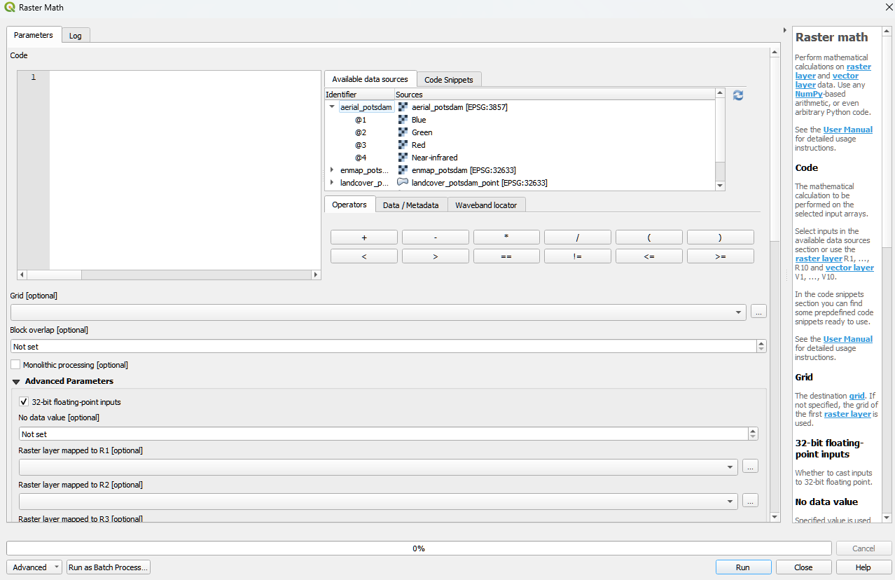
Raster math

The Raster math algorithm is a powerful raster calculator inspired by the QGIS Raster calculator, the GDAL Raster calculator and ENVI Band Math. In addition to those tools, the EnMAP-Box Raster math supports multi-band arrays, vector layer inputs, multi-line code fragments and metadata handling.

Usage

1. Start the algorithm from the Applications > Raster math menu or from the Processing Toolbox panel.

2. Specify a single-line expression or a multi-line code fragment to be evaluated inside the Code editor.

   Therefore, select raster bands or numeric vector fields from the Available data sources tab.

3. [Optional] Select the destination Grid. If not specified, the grid of the first raster layer is used. Note that a) all input raster bands are resampled and b) all input vector fields are rasterized into the destination grid before the calculation.

4. [Optional] In case you want to perform a spatial operation, be sure to select a proper Block overlap or select Monolithic processing, to avoid artefacts at the block edges.

5. [Optional] Note that all inputs are converted to 32-bit floating-point values by default.

6. [Optional] You can select up to 10 additional raster inputs R1, …, R10 and vector inputs V1, …, V10. Additionally, a list of raster inputs RS can be selected.

7. Select an Output raster layer file destination an click Run.

GUI

Single-line expressions

Use single-line expressions to evaluate simple numeric formulars.

Example - sum up 3 raster bands using the ‘+’ operator

A raster band is represented as a 2d numpy array and can be selected using the <layer name>@<band number> syntax.

aerial_potsdam@1 + aerial_potsdam@2 + aerial_potsdam@3

Example - sum up all bands of a raster using numpy.sum function

A raster is represented as a 3d numpy array and can be selected using the <layer name> syntax.

np.sum(enmap_potsdam, axis=0)

Use raster bands

An individual raster band can be accessed using the <layer name>@<band number> syntax, e.g. band number 42:

enmap_potsdam@42

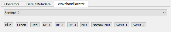
In case of a spectral raster, the band nearest to a target wavelength (in nanometers) can be selected using the <layer name>@<band number>nm syntax, e.g. NIR band at 865 nm:

enmap_potsdam@865nm

Note that prominent target wavelength from the Landsat/Sentinel-2 sensors can be selected inside the Waveband locator tab.

All raster bands can be accessed at once using the <layer name> syntax, e.g.:

enmap_potsdam

A band subset can be accessed using the <layer name>@<start>:<stop> syntax, e.g. band numbers 10 to 19:

enmap_potsdam@10:20  # note that 20 is not included

# Note that you can also create a band subset by indexing the the full band array.
# This has the slight disadvantage, that all bands are read into memory first.
enmap_potsdam[9:19]

Use vector fields

Individual vector fields can be accessed using the <layer name>@”<field name>” syntax, e.g.:

landcover_potsdam_polygon@"level_3_id"

Note that the vector field is automatically rasterized into the destination Grid.

Use raster/vector masks

A raster mask, is a predefined boolean array, which evaluates to False for every pixel containing the no data value, nan or inf. All other pixel evaluate to True.

Use the <layer name>Mask syntax to access the 3d binary mask for all bands, and the <layer name>Mask@<band number> syntax for a 2d single band mask.

2d mask array for a single band: enmap_potsdamMask@655nm

A vector mask is a predefined boolean array, which evaluates to True for every pixel covered by a geometry. All other pixel evaluate to False. Use the <layer name> syntax to access the 2d binary mask.

2d mask array for a vector layer: landcover_potsdam_polygon

Example - mask a raster using a polygon-vector

enmap_potsdam * landcover_potsdam_polygon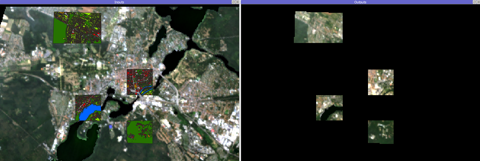

Note that the output raster is correctly masked, but we haven’t set an appropriate no data value, nor have we taken care of wavelength information or any other metadata. To properly do this, we need to use multi-line code fragments.

Blockwise vs. monolithic processing

The computation is done block-wise by default to be memory efficient. The actual block size depends on the system memory. In rare cases it may be helpful to get some information about the current block, using the special variable block.

• get the current block extent: block.extent:

  <QgsRectangle: 380952.36999999999534339 5808372.34999999962747097, 387552.36999999999534339 5820372.34999999962747097>
  

• get the current block x/y offset: block.xOffset, block.yOffset:

  0, 0
  

• get the current block x/y size: block.width, block.height:

  220, 400
  

If the computation involves a spatial operation, e.g. a spatial convolution filter with a kernel, be sure to also specify a proper Block overlap. E.g. for a 5x5 kernel, set at least a block overlap of 2 pixel.

In cases where the spatial operation is not locally limitted to a fixed spatial neightbourhood, e.g. region growing or segmentation, Monolithic processing can be activated, where all data is processed in one big block.

Multi-line code fragments

To enable more complex computations, multiple outputs and metadata handling, we can use multi-line code fragments.

Example - calculate the NDVI index

In this example we first specify _nir and _red variables to then calculate the _ndvi, which we pass to the special outputRaster identifier, that is associated with the Output raster layer:

nir_ = enmap_potsdam@865nm
red_ = enmap_potsdam@655nm
ndvi_ = (nir_ - red_) / (nir_ + red_)
outputRaster = ndvi_

The underscore postfix _ marks the nir_, red_ and ndvi_ variables as temporary. Instead of nir_ we can also use _nir, tmp_nir or temp_nir.

The explicite assignment outputRaster = ndvi_ can be avoided, by selecting an Output raster layer file destination, where the file basename (without extension) matches the variable name, e.g. c:/ndvi.tif:

nir_ = enmap_potsdam@865nm
red_ = enmap_potsdam@655nm
ndvi = (nir_ - red_) / (nir_ + red_)  # ndvi matches with c:/ndvi.tif

If the file basename isn’t matching correctly, you will get the following error message inside the Log panel:

The following layers were not correctly generated.
• C:/Users/Andreas/AppData/Local/Temp/processing_BVyjbt/3a6c795d9a594937acf441c5a372f448/outputRaster.tif
You can check the 'Log Messages Panel' in QGIS main window to find more information about the execution of the algorithm.

Instead of using temporary variables, you can also just delete unwanted variables as a last step:

nir = enmap_potsdam@865nm
red = enmap_potsdam@655nm
ndvi = (nir - red) / (nir + red)

del nir, red  # delete temporary variables manually

Example - calculate multiple outputs

To calculate multiple outputs, just define multiple non-temporary variables:

N = enmap_potsdam@865nm / 1e4  # EVI needs data scaled to 0-1 range
R = enmap_potsdam@655nm / 1e4
B = enmap_potsdam@482nm / 1e4

ndvi = (N - R) / (N + R)
evi = 2.5 * (N - R) / (N + 6 * R - 7.5 * B + 1)

del N, R, B

Note that you can only specify the file destination of one of the outputs, e.g. by setting Output raster layer to c:/results/ndvi.tif or c:/results/evi.tif. The other output is written into the same directory as a GeoTiff with the basename matching the variable name c:/results/<basename>.tif.

You may also keep the default file destination [Save to temporary file] as is, to write all outputs into a temp folder. In this case, it is fine to just ignore the error message:

The following layers were not correctly generated.
• C:/Users/Andreas/AppData/Local/Temp/processing_BVyjbt/3a6c795d9a594937acf441c5a372f448/outputRaster.tif
You can check the 'Log Messages Panel' in QGIS main window to find more information about the execution of the algorithm.

Metadata handling

You have full access to the underlying raster metadata like:

• band no data value: enmap_potsdam.noDataValue(bandNo=1):

  -99.0
  

• band name: enmap_potsdam.bandName(bandNo=1):

  band 8 (0.460000 Micrometers)
  

• band-level metadata dictionary: enmap_potsdam.metadata(bandNo=1):

  {'': {'wavelength': '0.460000', 'wavelength_units': 'Micrometers'}}
  

• band-level metadata item: enmap_potsdam.metadataItem(key='wavelength_units', domain='', bandNo=1):

  Micrometers
  

• dataset-level metadata dictionary: enmap_potsdam.metadata():

  {'IMAGE_STRUCTURE': {'INTERLEAVE': 'BAND'}, '': {'wavelength_units': 'Micrometers'}, 'ENVI': {'acquisition_time': '2009-08-20T09:44:50', 'bands': '177', 'band_names': ['band 8', 'band 9', 'band 10', 'band 11', 'band 12', 'band 13', 'band 14', 'band 15', 'band 16', 'band 17', 'band 18', 'band 19', 'band 20', 'band 21', 'band 22', 'band 23', 'band 24', 'band 25', 'band 26', 'band 27', 'band 28', 'band 29', 'band 30', 'band 31', 'band 32', 'band 33', 'band 34', 'band 35', 'band 36', 'band 37', 'band 38', 'band 39', 'band 40', 'band 41', 'band 42', 'band 43', 'band 44', 'band 45', 'band 46', 'band 47', 'band 48', 'band 49', 'band 50', 'band 51', 'band 52', 'band 53', 'band 54', 'band 55', 'band 56', 'band 57', 'band 58', 'band 59', 'band 60', 'band 61', 'band 62', 'band 63', 'band 64', 'band 65', 'band 66', 'band 67', 'band 68', 'band 69', 'band 70', 'band 71', 'band 72', 'band 73', 'band 74', 'band 75', 'band 76', 'band 77', 'band 91', 'band 92', 'band 93', 'band 94', 'band 95', 'band 96', 'band 97', 'band 98', 'band 99', 'band 100', 'band 101', 'band 102', 'band 103', 'band 104', 'band 105', 'band 106', 'band 107', 'band 108', 'band 109', 'band 110', 'band 111', 'band 112', 'band 113', 'band 114', 'band 115', 'band 116', 'band 117', 'band 118', 'band 119', 'band 120', 'band 121', 'band 122', 'band 123', 'band 124', 'band 125', 'band 126', 'band 127', 'band 144', 'band 145', 'band 146', 'band 147', 'band 148', 'band 149', 'band 150', 'band 151', 'band 152', 'band 153', 'band 154', 'band 155', 'band 156', 'band 157', 'band 158', 'band 159', 'band 160', 'band 161', 'band 162', 'band 163', 'band 164', 'band 165', 'band 166', 'band 167', 'band 168', 'band 195', 'band 196', 'band 197', 'band 198', 'band 199', 'band 200', 'band 201', 'band 202', 'band 203', 'band 204', 'band 205', 'band 206', 'band 207', 'band 208', 'band 209', 'band 210', 'band 211', 'band 212', 'band 213', 'band 214', 'band 215', 'band 216', 'band 217', 'band 218', 'band 219', 'band 220', 'band 221', 'band 222', 'band 223', 'band 224', 'band 225', 'band 226', 'band 227', 'band 228', 'band 229', 'band 230', 'band 231', 'band 232', 'band 233', 'band 234', 'band 235', 'band 236', 'band 237', 'band 238', 'band 239'], 'byte_order': '0', 'coordinate_system_string': ['PROJCS["UTM_Zone_33N"', 'GEOGCS["GCS_WGS_1984"', 'DATUM["D_WGS_1984"', 'SPHEROID["WGS_1984"', '6378137.0', '298.257223563]]', 'PRIMEM["Greenwich"', '0.0]', 'UNIT["Degree"', '0.0174532925199433]]', 'PROJECTION["Transverse_Mercator"]', 'PARAMETER["False_Easting"', '500000.0]', 'PARAMETER["False_Northing"', '0.0]', 'PARAMETER["Central_Meridian"', '15.0]', 'PARAMETER["Scale_Factor"', '0.9996]', 'PARAMETER["Latitude_Of_Origin"', '0.0]', 'UNIT["Meter"', '1.0]]'], 'data_ignore_value': '-99', 'data_type': '2', 'description': ['EnMAP02_potsdam_Urban_Gradient_2009.bsq', 'http://doi.org/10.5880/enmap.2016.008', 'spectral and spatial subset'], 'file_type': 'ENVI Standard', 'fwhm': ['0.005800', '0.005800', '0.005800', '0.005800', '0.005800', '0.005800', '0.005800', '0.005800', '0.005800', '0.005800', '0.005900', '0.005900', '0.006000', '0.006000', '0.006100', '0.006100', '0.006200', '0.006200', '0.006300', '0.006400', '0.006400', '0.006500', '0.006600', '0.006600', '0.006700', '0.006800', '0.006900', '0.006900', '0.007000', '0.007100', '0.007200', '0.007300', '0.007300', '0.007400', '0.007500', '0.007600', '0.007700', '0.007800', '0.007900', '0.007900', '0.008000', '0.008100', '0.008200', '0.008300', '0.008400', '0.008400', '0.008500', '0.008600', '0.008700', '0.008700', '0.008800', '0.008900', '0.008900', '0.009000', '0.009100', '0.009100', '0.009200', '0.009300', '0.009300', '0.009400', '0.009400', '0.009500', '0.009500', '0.009600', '0.009600', '0.009600', '0.009600', '0.009700', '0.009700', '0.009700', '0.011800', '0.011900', '0.012100', '0.012200', '0.012400', '0.012500', '0.012700', '0.012800', '0.012900', '0.013100', '0.013200', '0.013300', '0.013400', '0.013500', '0.013600', '0.013700', '0.013800', '0.013900', '0.014000', '0.014000', '0.014100', '0.014100', '0.014200', '0.014200', '0.014300', '0.014300', '0.014300', '0.014400', '0.014400', '0.014400', '0.014400', '0.014400', '0.014400', '0.014400', '0.014400', '0.014400', '0.014400', '0.013700', '0.013600', '0.013600', '0.013500', '0.013500', '0.013400', '0.013400', '0.013300', '0.013200', '0.013200', '0.013100', '0.013100', '0.013000', '0.012900', '0.012900', '0.012800', '0.012800', '0.012700', '0.012700', '0.012600', '0.012500', '0.012500', '0.012400', '0.012400', '0.012300', '0.010900', '0.010800', '0.010800', '0.010700', '0.010700', '0.010600', '0.010600', '0.010500', '0.010500', '0.010400', '0.010400', '0.010400', '0.010300', '0.010300', '0.010200', '0.010200', '0.010100', '0.010100', '0.010100', '0.010000', '0.010000', '0.009900', '0.009900', '0.009900', '0.009800', '0.009800', '0.009700', '0.009700', '0.009700', '0.009600', '0.009600', '0.009600', '0.009500', '0.009500', '0.009400', '0.009400', '0.009400', '0.009300', '0.009300', '0.009300', '0.009200', '0.009200', '0.009100', '0.009100', '0.009100'], 'header_offset': '0', 'interleave': 'bsq', 'lines': '400', 'reflectance_scale_factor': '10000', 'samples': '220', 'sensor_type': 'Unknown', 'wavelength': ['0.460000', '0.465000', '0.470000', '0.475000', '0.479000', '0.484000', '0.489000', '0.494000', '0.499000', '0.503000', '0.508000', '0.513000', '0.518000', '0.523000', '0.528000', '0.533000', '0.538000', '0.543000', '0.549000', '0.554000', '0.559000', '0.565000', '0.570000', '0.575000', '0.581000', '0.587000', '0.592000', '0.598000', '0.604000', '0.610000', '0.616000', '0.622000', '0.628000', '0.634000', '0.640000', '0.646000', '0.653000', '0.659000', '0.665000', '0.672000', '0.679000', '0.685000', '0.692000', '0.699000', '0.706000', '0.713000', '0.720000', '0.727000', '0.734000', '0.741000', '0.749000', '0.756000', '0.763000', '0.771000', '0.778000', '0.786000', '0.793000', '0.801000', '0.809000', '0.817000', '0.824000', '0.832000', '0.840000', '0.848000', '0.856000', '0.864000', '0.872000', '0.880000', '0.888000', '0.896000', '0.915000', '0.924000', '0.934000', '0.944000', '0.955000', '0.965000', '0.975000', '0.986000', '0.997000', '1.007000', '1.018000', '1.029000', '1.040000', '1.051000', '1.063000', '1.074000', '1.086000', '1.097000', '1.109000', '1.120000', '1.132000', '1.144000', '1.155000', '1.167000', '1.179000', '1.191000', '1.203000', '1.215000', '1.227000', '1.239000', '1.251000', '1.263000', '1.275000', '1.287000', '1.299000', '1.311000', '1.323000', '1.522000', '1.534000', '1.545000', '1.557000', '1.568000', '1.579000', '1.590000', '1.601000', '1.612000', '1.624000', '1.634000', '1.645000', '1.656000', '1.667000', '1.678000', '1.689000', '1.699000', '1.710000', '1.721000', '1.731000', '1.742000', '1.752000', '1.763000', '1.773000', '1.783000', '2.044000', '2.053000', '2.062000', '2.071000', '2.080000', '2.089000', '2.098000', '2.107000', '2.115000', '2.124000', '2.133000', '2.141000', '2.150000', '2.159000', '2.167000', '2.176000', '2.184000', '2.193000', '2.201000', '2.210000', '2.218000', '2.226000', '2.234000', '2.243000', '2.251000', '2.259000', '2.267000', '2.275000', '2.283000', '2.292000', '2.300000', '2.308000', '2.315000', '2.323000', '2.331000', '2.339000', '2.347000', '2.355000', '2.363000', '2.370000', '2.378000', '2.386000', '2.393000', '2.401000', '2.409000'], 'wavelength_units': 'Micrometers', 'y_start': '24', 'z_plot_titles': ['wavelength [!7l!3m]!N', 'reflectance [*10000]']}}}
  

• dataset-level metadata item: enmap_potsdam.metadataItem(key='wavelength_units', domain=''):

  Micrometers
  

In general, all the methods provided by the RasterReader class can be used: https://github.com/EnMAP-Box/enmap-box/blob/main/enmapboxprocessing/rasterreader.py

For the outputs, you can use all the methods provided by the RasterWriter class: https://github.com/EnMAP-Box/enmap-box/blob/main/enmapboxprocessing/rasterwriter.py

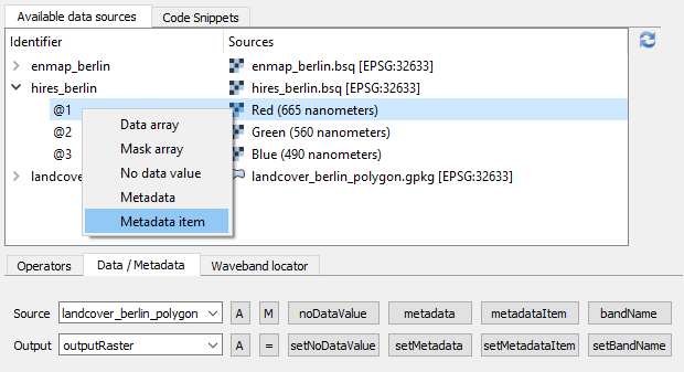
Also note the shortcuts inside the Available data sources tab context menu and the Data / Metadata tab.

Example - calculate the NDVI index and set up metadata properly

This example shows how to properly calculate the NDVI index, masking no data pixel and set up output metadata:

# find bands
red = enmap_potsdam@655nm
nir = enmap_potsdam@865nm

# calculate NDVI
ndvi = (nir - red) / (nir + red)

# mask no data region
noDataValue = -9999
ndvi[~enmap_potsdamMask@655nm] = noDataValue
ndvi[~enmap_potsdamMask@865nm] = noDataValue

# set no data value and band name
ndvi.setNoDataValue(noDataValue)
ndvi.setBandName('NDVI', bandNo=1)

# clean up temp variables
del red, nir

Example - copy raster data and metadata

This example shows how to properly copy a raster data and metadata:

# copy data
copy = enmap_potsdam

# copy metadata
copy.setMetadata(enmap_potsdam.metadata())
for bandNo in enmap_potsdam.bandNumbers():
    copy.setMetadata(enmap_potsdam.metadata(bandNo), bandNo)
    copy.setBandName(enmap_potsdam.bandName(bandNo), bandNo)
    copy.setNoDataValue(enmap_potsdam.noDataValue(bandNo), bandNo)

Input raster lists

For some operations it may be necessary to enter an arbitrary large list of rasters. In this case, use the Raster layers mapped to RS.

Example - average a list of rasters

np.mean(RS, axis=0)

As for normal input raster, use the RSMask syntax to access the binary no data value masks.

Regression Dataset Manager

todo

Regression Workflow (deprecated)

See also

Have a look at the Biomass Mapping Tutorial for a use case example of the Regression Workflow Application.

Input Parameters:

• Training Inputs

  • Raster: Specify input raster based on which samples will be drawn for training a regressor.

  • Reference: Specify vector or raster dataset with reference information (regression target). In case of vector input, dataset has to have a numeric column in the attribute table with a target variable of interest. This vector dataset is rasterized/burned on-the-fly onto the grid of the input raster in order to extract the sample. If the vector source is a polygon dataset, all pixels will be drawn which intersect the polygon.

  • Attribute: Attribute field in the reference vector layer which contains the regression target variable.

• Sampling

  • Number of Strata : Specify the desired number of strata sampling. If you don’t want to use stratified sampling, just enter 1.

  • Min & Max: Defines the value range in which samples should be drawn.

  • Sample size : Specify the sample size per stratum, either relative in percent or in absolute pixel counts.

    Every stratum is listed below with the value range that is covered by this stratum depicted in square brackets (e.g., Stratum 1: [1.0, 4.33]). Furthermore, you can see and alter the number of pixels/samples for each stratum using the spinboxes.

  • Save sample: Activate this option and specify an output path to save the sample as a raster.

• Training

  • In the Regressor dropdown menu you can choose different regressors (e.g. Random Forest, Support Vector Regression, Kernel Ridge Regression)

  • Model parameters: Specify the parameters of the selected regressor.

    Hint

    Scikit-learn python syntax is used here, which means you can specify model parameters accordingly. Have a look at the scikit-learn documentation on the individual parameters, e.g. for the RandomForestRegressor

  • Save model: Activate this option to save the model file (.pkl) to disk.

• Mapping

  • Input Raster: Specify the raster you would like to apply the trained regressor to (usually -but not necessarily- this is the same as used for training)

• Cross-validation Accuracy Assessment

  • Cross-validation with n-folds : Activate this setting to assess the accuracy of the regression by performing cross validation. Specify the desired number of folds (default: 3). HTML report will be generated at the specified output path.

Run the regression workflow

Once all parameters are entered, press the button to start the regression workflow.

Spectral Index Creator

todo