This tutorial give an introduction into the use of spectral libraries in the EnMAP-Box.
It is designed for EnMAP-Box 3.14 or higher. Minor changes may be present in subsequent versions, such as modified menu labels or added parameter options.
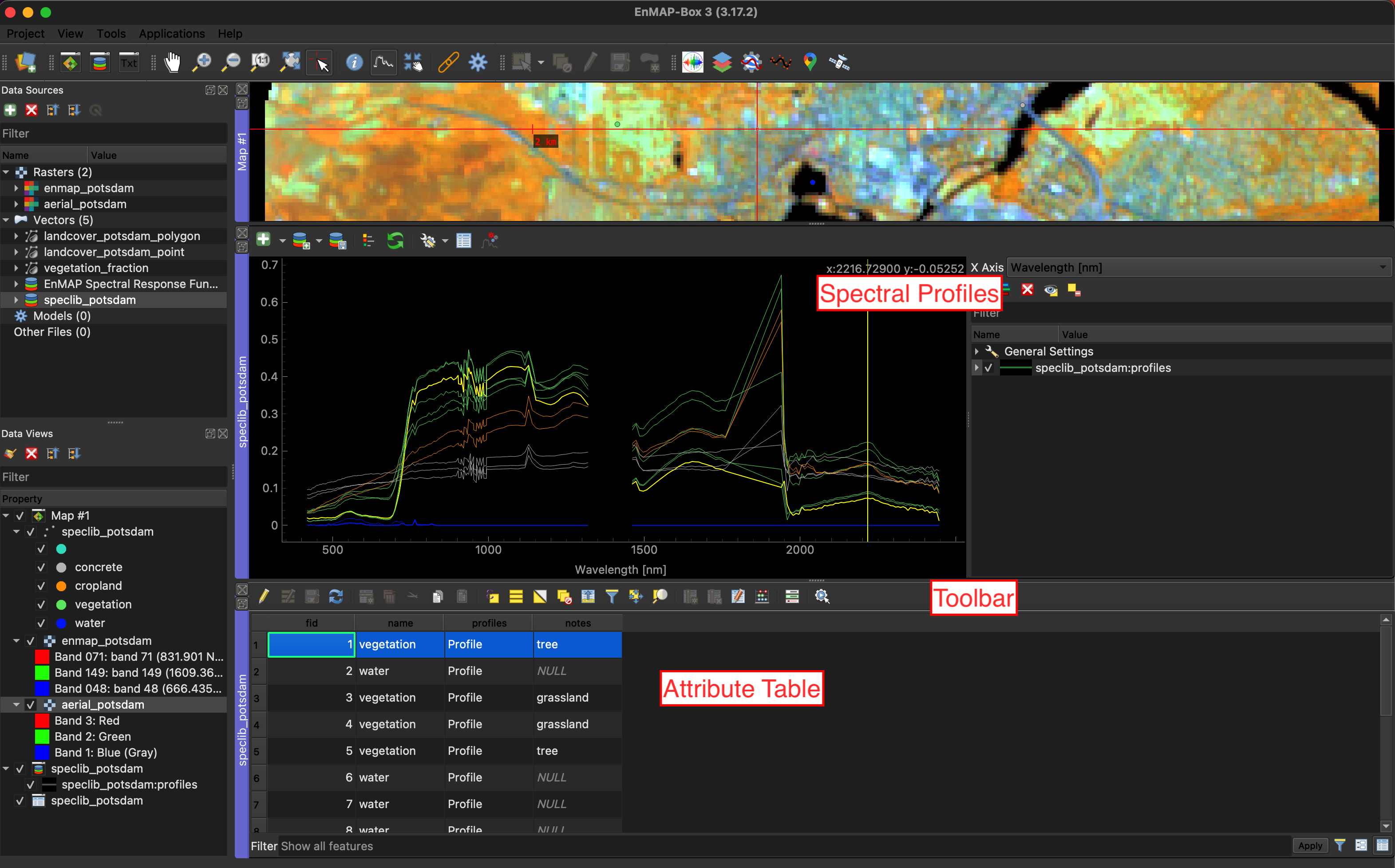
Launch QGIS and click the icon in the toolbar to open the EnMAP-Box. The EnMAP-Box GUI comprises a Menu and a Toolbar, panels for Data Sources and Data Views, and the QGIS Processing Toolbox, which includes the EnMAP-Box Processing Algorithms.
Most function in toolbar you already know from the normal QGIS attribute table.
The Spectral Library viewer just adds extra tools to create, edit and export profiles.
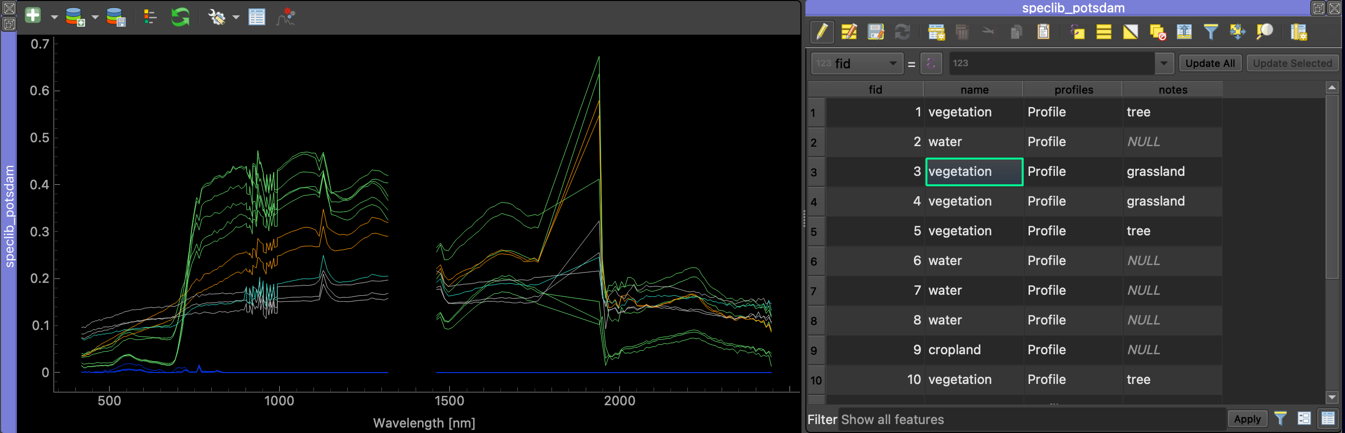
The spectral profiles window shows the spectral profiles of the features, in our case points with attributes,
that are collected in the spectral library.
There is a button to show or hide the properties of the spectral profile window.
The attribute table shows the none-spatial information for each feature in a row.
Let’s have a closer look at the toolbar:
While being in the editing mode , additional options are unlocked to modify your attribute table:
Let’s open a spectral library that provides coordinates for each spectral profile:
Open a new map view with the enmap_potsdam image.
Download and extract the speclib_potsdam.zip.
The zip file contains the speclib_potsdam.gpkg with the data and a speclib_potsdam.qml style file
that tells QGIS and the EnMAP-Box how to visualize it.
Drag and drop the speclib_potsdam.gpkg to the EnMAP-Box Data Source Panel.
Use the context menu Open Spectral Library Viewer to visualize the spectral profiles.
Use the Map View context menu to add the speclib_potsdam vector layer
Fig. 6.2.1 Opening the speclib_potsdam.gpkg library in a Spectral Library View and a Map View.
In this introduction we like to collect additional profiles for the following classes:
Concrete
Cropland
Vegetation
Water
Add the areal_potsdam DOP image to the Map View. It gives us a better understanding
which classes are covered by a single EnMAP pixel
Search for areas with that kind of surface coverage.
Next, click on then on . When you click on a point in the image,
a spectral profile will be shown on top of the other profiles in the Spectral Library View.
Simultaneously the Spectral Profile Source Panel opens on the right.
By default, profiles are collected from the top-most raster layer.
The Spectral Profile Source Panel allows to change this and control how profiles are collected.
It will be explained in more detail below.
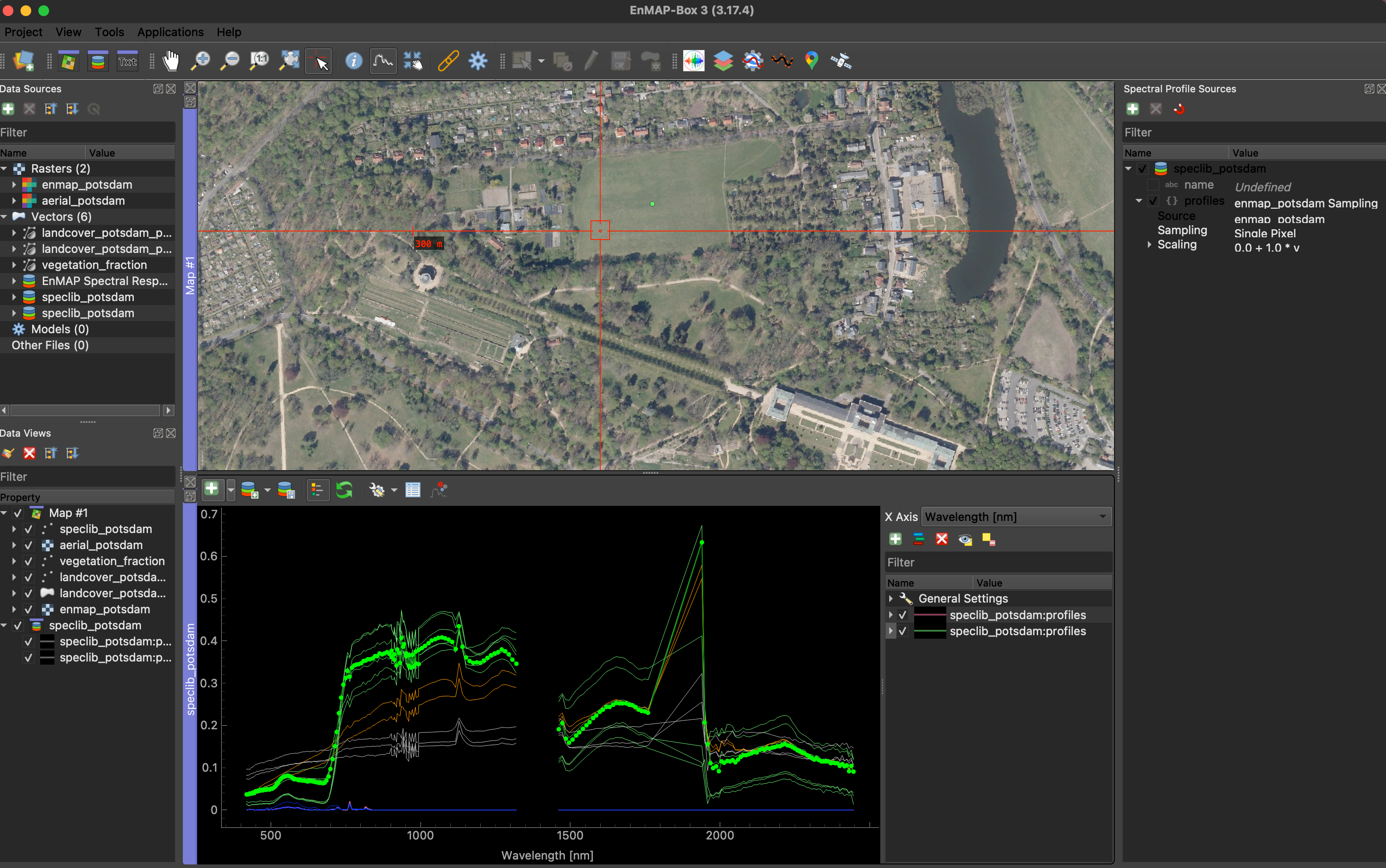
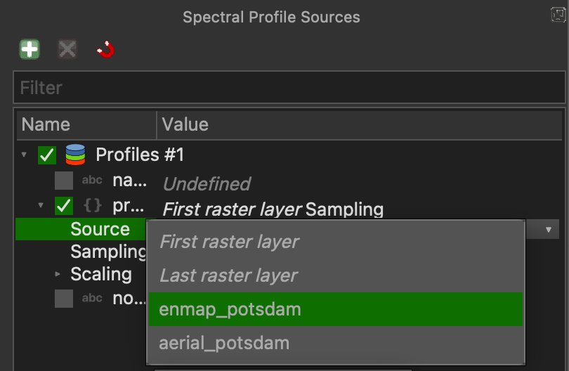
In order to collect profiles from the EnMAP image only, select enmap_potsdam as profile source .
Fig. 6.2.2 Collecting spectral profiles from an EnMAP image.
Profiles will now be collected from the EnMAP image and the aerial image
will make the classification easier.
To see the EnMAP pixel size underneath, open the Map View context menu, then click on Crosshair, Pixel Grid and select enmap_potsdam.
When you select a location, a profile candidate is added to the spectral library vector layer. However, this entry is temporary. If you select a new location without clicking the Add button , the current candidate will be automatically deleted and replaced by the new selection. To permanently keep a profile in the library, you must click .
With the new spectral profiles candidates are added automatically.
The Spectral Profile Source panel allows you to (i) specify how spectral profiles are collected from the raster data, (ii) how these profiles can be described in other attribute fields, and how temporary profiles will be displayed.
If you select and without having a Spectral Library View opened, the Spectral Profiles Source panel will open one automatically when you click on a pixel in the map for the first time.
To open the Spectral Profiles Source panel manually, click on View in the menu, select Panels, and then choose Spectral Profiles Source.
Fig. 6.2.6 The Spectral Profile Source panel (right) specifies how profiles are collected, described
and displayed when overlaid in a linked Spectral Library View.
To add a new relation that describes raster image sources and spectral library vector fields, click on .
First, let’s focus on the definition of how spectral profiles are collected:
Profiles specifies how the profiles are stored in the Profiles field in the spectral library attribute table.
You can specify the raster source from which the profile is sampled. Choose enmap_potsdam.
Style lets you specify how the sampled profiles are displayed when overlaid in the Spectral Library view.
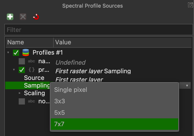
Sampling can be used to define how the profiles are sampled around the mouse coordinate.
Scaling allows to account for scaling differences between the profile source and profiles in your spectral library.
Now let’s look at how other attributes, e.g. integer, float or text values, can be created.
We like to generate a profile name automatically.
Ensure that the notes row is checked.
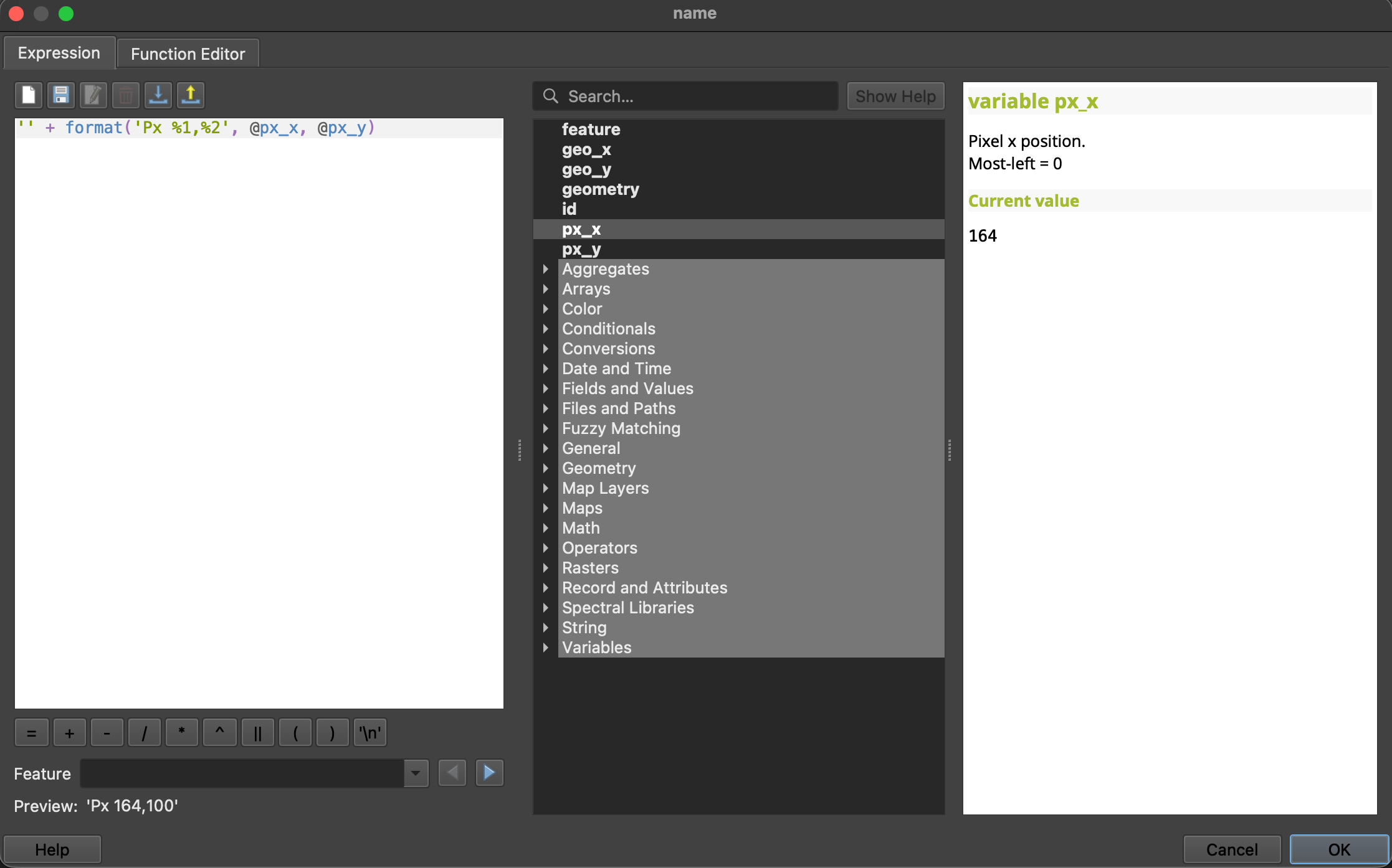
Double Click to edit, or open the Expression Builder with ε
With the Expression Builder you can create expressions that dynamically generate attributes.
Write ''+format('Px%1,%2',@px_x,@px_y) to generate a string that includes the pixel position, as in Px23,24.
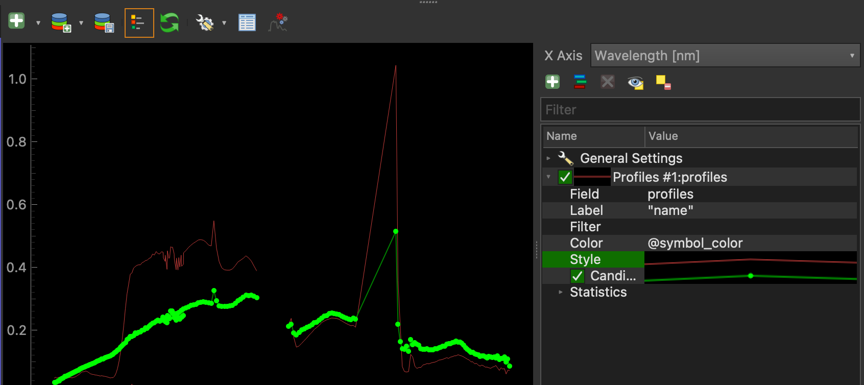
The profile visualization settings allow you to change profile color, line and symbol styles.
By default, profiles in the spectral library use the @symbol_color that is used in the map visualization.
In that case you can use the layer legend to show or hide groups of profiles. Changing the layer rendering in the map will change the profile colors too.
You can define your own colors and even use the expression builder to generate colors based profile attributes
Temporarily profile candidates use the style that is defined in the Spectra Profile Source Panel.
Go to the Layer Properties of your spectral library in the Data Views panel. With Symbology you can set the colors.
Fig. 6.2.8 The vector layer symbology panel defines the feature symbols…
Choose Categorized, for Value, select the column according to which the classes are to be differentiated. Click Classify.
You can change the colors by double-clicking on the color you want to change.
Click OK. Now your spectra have different colors and your graph is more clear.
Fig. 6.2.9 … whose colors can be used as profile color.
Click the “+” button to create a new profile visualization.
This way you can differentiate profiles by other means than the vector layer map symbology.
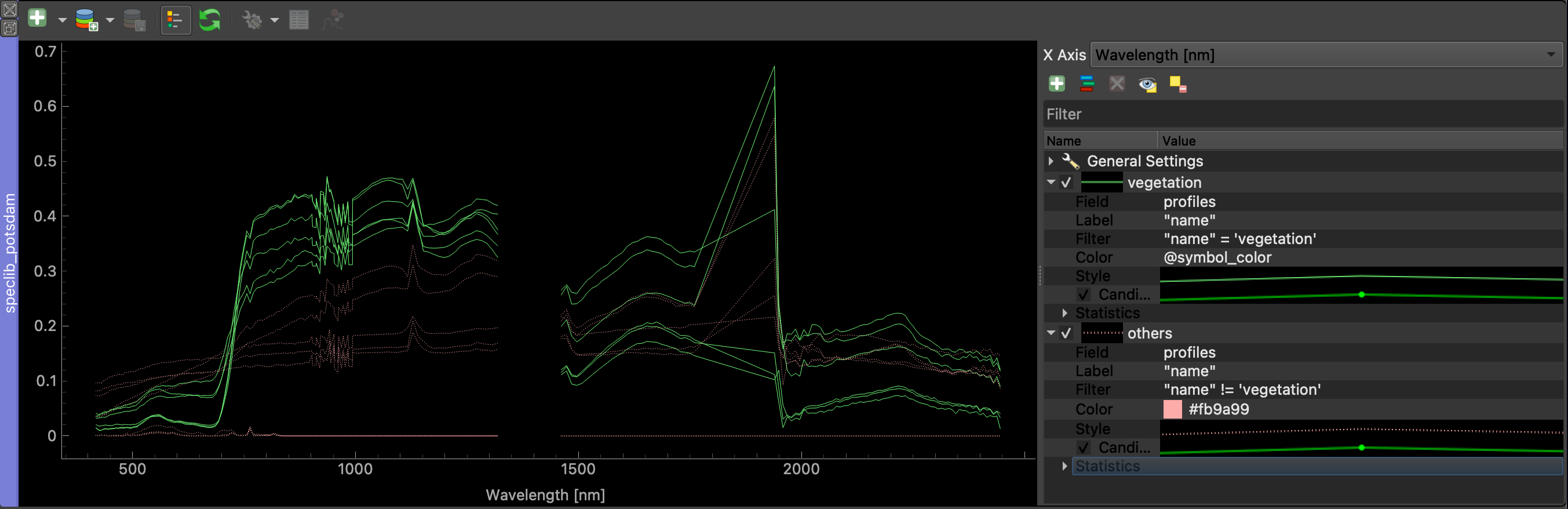
Create a group for vegetation that uses the filter expression “name” = ‘vegetation’. Double click on entries in the Value column to edit the visualization name or define filter expressions.
Create a group for Other profiles with filter expression “name” != ‘vegetation’
Style both groups differently, e.g. by showing non-vegetation in dotted lines
Fig. 6.2.10 Using multiple visualization groups allows for fine-tuned profiles styles
QGIS uses a transaction model to save changes. Modification are saved in an edit-buffer.
To save changes permanently to the data source requires to:
click the save edits button , or
disable the edit mode . If changes are available, this opens the Stop Editing dialog
Press Yes to save your edits, or
Press No to rollback all modifications.
Warning
Be aware that savings may be made to in-memory data sources. These data sources are lost when closing the EnMAP-Box or QGIS. For example a new (and empty) Spectral Library Viewer uses an in-memory as data source.
To save such spectral libraries permanently requires to export them into persistant data formats, like a GeoPackage file (see below Export Spectral Profiles)
To import profiles from a Raster Layer, drag and drop your raster file and a vector file
with locations to extract the raster profiles into a new map window.
Open Import Spectral Profiles window and choose Raster Layer
Select the raster layer from which you like to import profiles
Select the vector layer that specifies the profile locations
Specify which other raster and vector attributes will be written to the Spectral Library.
To import the columns of your choice, click on and select the columns.
To import a Raster Layer, drag and drop your raster file into a new map window.
When you open the Import Spectral Profiles window and select Raster Layer, the Raster File will automatically appear in the Options. If multiple Raster Layers are open, you can choose one.
To import the columns of your choice, click on and select the columns.
Click OK
Fig. 6.4.3 Importing spectral profiles from a raster layer and a vector layer that specifies the profile locations.
You might already know the QGIS field calculator and have used it to calculate values of vector layer attributes. We can use it to extract or modify spectral profiles as well:
Open the enmap_potsdam raster layer and the landcover_potsdam_point layer in a new map window.
Click on the landcover_potsdam_point with the right mouse button and select Open Spectral Library Viewer. A new spectral library window opens.
The points are in the attribute table, but not yet associated with any spectral information.
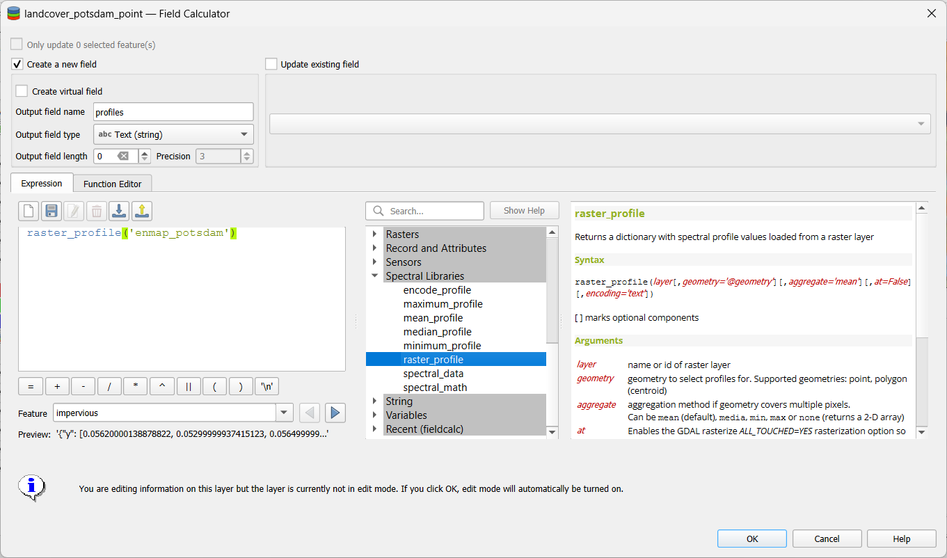
Open the Field Calculator and make the following settings to link the points to spectral profiles:
Check Create a new field
Set an Output field name profiles
Output field type: Text(string), with Text length = 0 (unlimited)
In the expression field write: raster_profile('enmap_potsdam')
Click OK to calculate your profiles and make them visible in the attribute table now.
Click on the landcover_potsdam_point with the right mouse button and select Open Spectral Library Viewer. A new spectral library window opens. The points are in the attribute table, but not yet associated with any spectral information.
Fig. 6.4.4 Any vector layer can be opened in a Spectral Library View and edited with the QGIS Field Calculator.
To link the points to spectral profiles, follow these steps in the Field Calculator:
Tick Create a new field
Set an output field name
Output field type: Text(string)
In the expression field write the command: raster_profile(‘enmap_potsdam’) to connect the points to the spectral information.
Click OK and your profiles are visible in the attribute table now.
Fig. 6.4.5 EnMAP-Box functions to manage spectral profiles with the QGIS Field Calculator
Fig. 6.4.6 Creating spectral profiles using the QGIS Field Calculator.
To show the spectral profiles, click on Update Profiles on the left hand side of the toolbar.
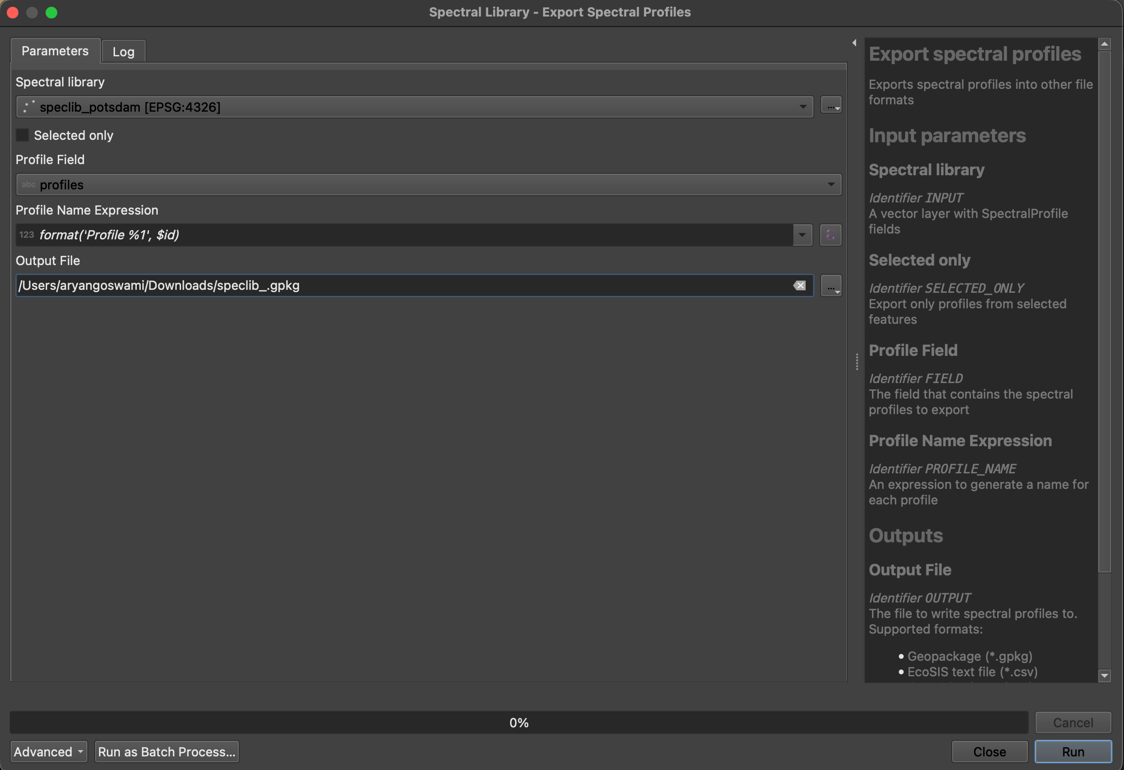
Click on the symbol. The Export Spectral Library window will open.
Fig. 6.5.1 Dialog to export spectral profiles into a new GeoPackage file.
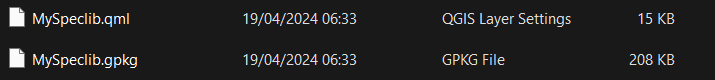
Export the spectral library as *.gpkg and choose a file path and layer name.
Two files are saved: the geopackage file which contains the points and attributes, including the spectral profiles, and an QML file with styling information.
The new speclib data source is automatically added to the EnMAP-Box data sources and can be opened in QGIS as well
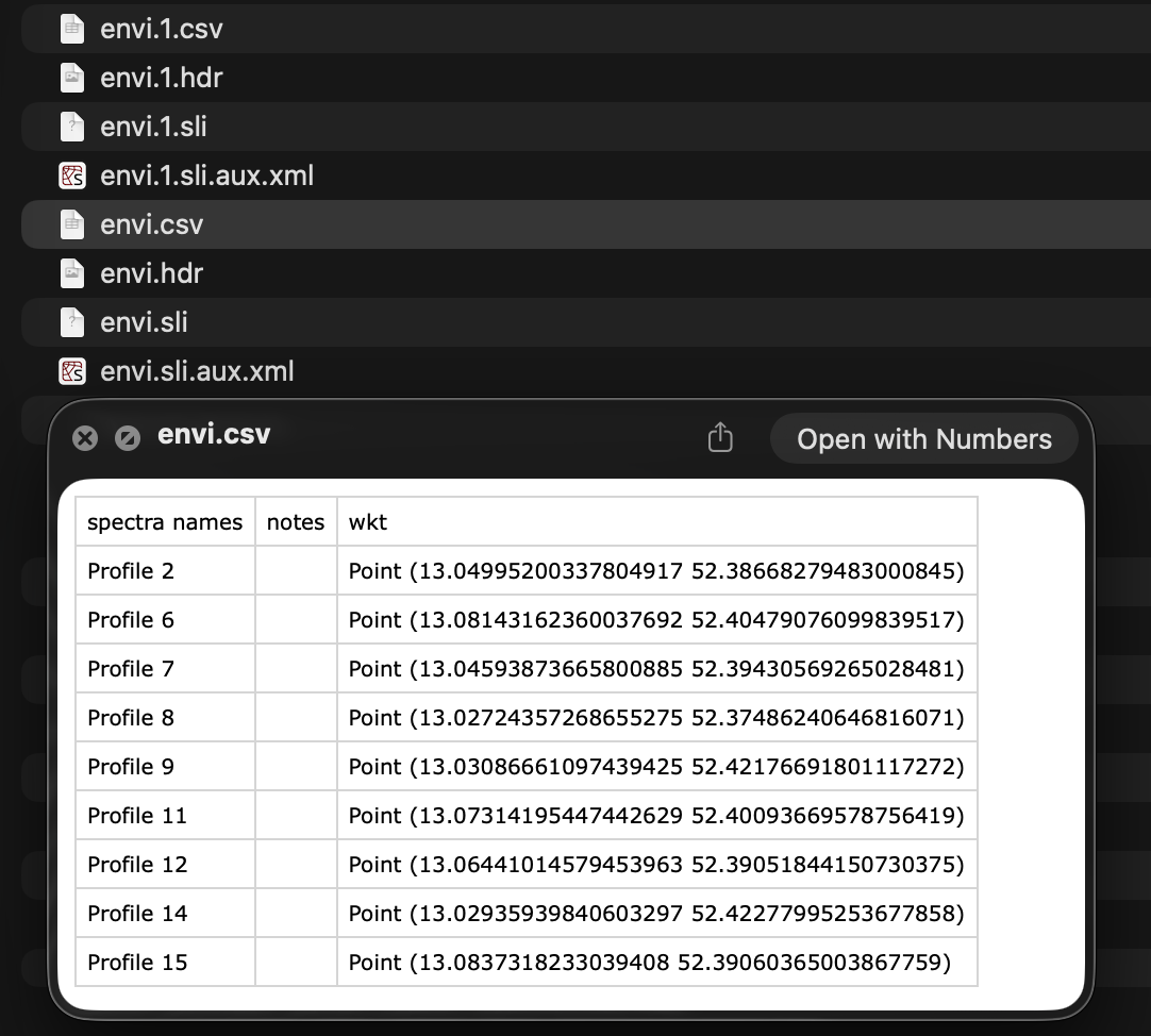
Now export the spectral library as a ENVI Spectral Library*.sli.
Choose a field from which to export the profiles and a field that contains the profile names.
Fig. 6.5.2 Export spectral profiles as ENVI Spectral Library.
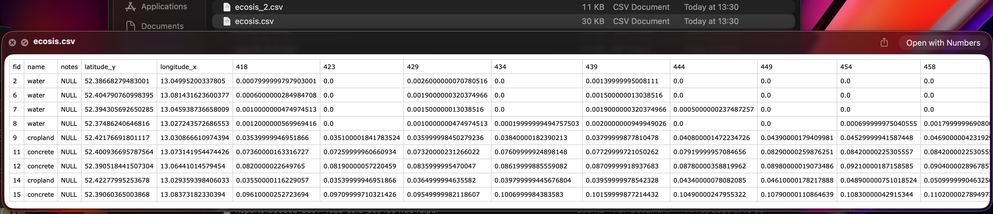
The new ENVI Spectral Library (*.sli) is accompanied by a .csv file that lists additional values from, like the point coordinates in WKT notation.
Note
Our spectral library could contain profiles from different sensors in the same field, but
the ENVI spectral library format does not allow to save profiles with a differing number of bands. In that case the EnMAP-Box will create multiple *.sli file, one for each set of profiles that are similar in the number of bands and wavelengths.
Now export the spectral library as a EcoSIS Spectral Library*.csv.
Choose a field from which to export the profiles and for names you can choose the field that contains names or you can also use a profile name expression to generate names.
Fig. 6.5.3 Export spectral profiles as EcoSIS Spectral Library.
 icon in the toolbar to open the EnMAP-Box. The EnMAP-Box GUI comprises a Menu and a Toolbar, panels for Data Sources and Data Views, and the QGIS Processing Toolbox, which includes the EnMAP-Box Processing Algorithms.
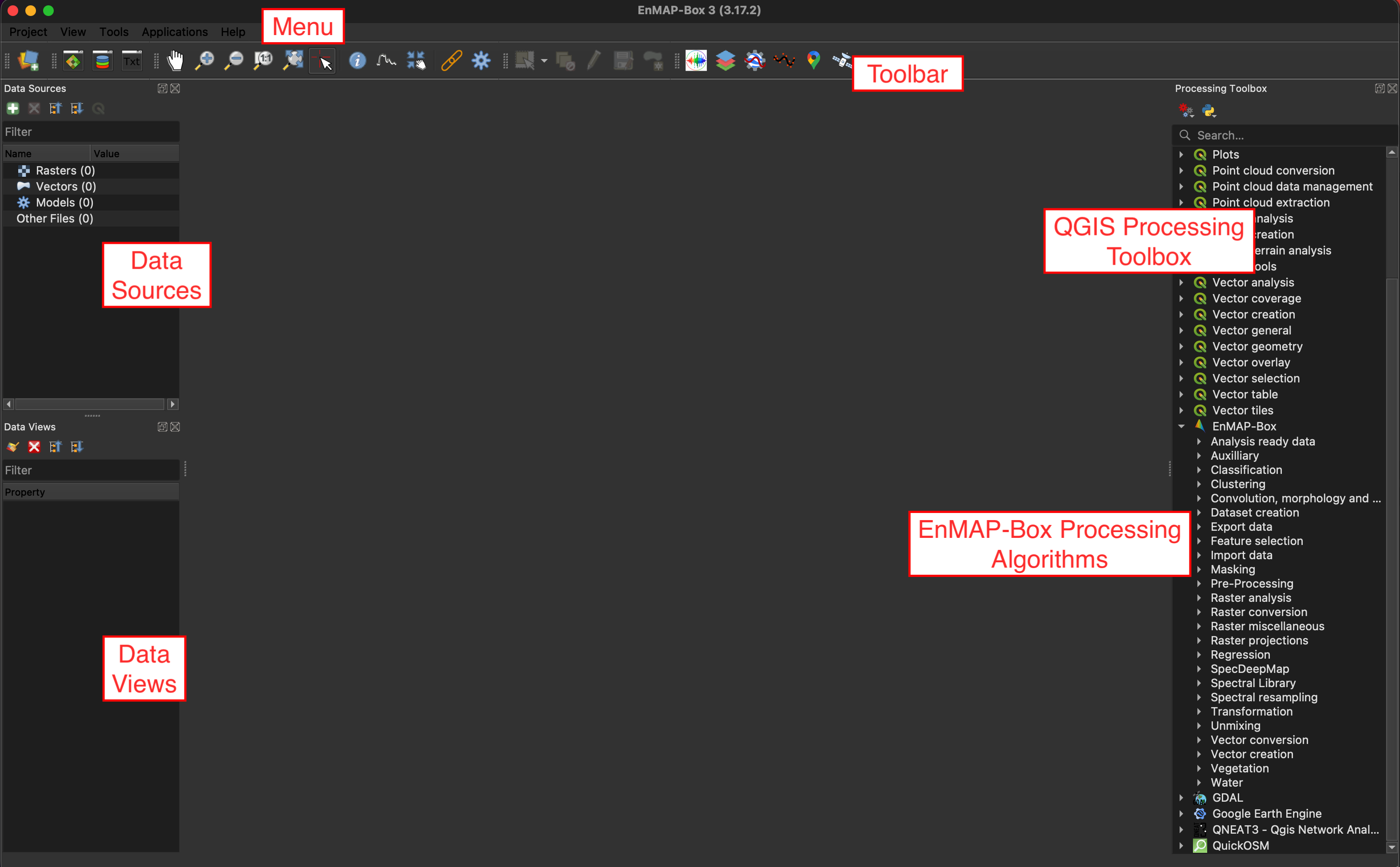

 , additional options are unlocked to modify your attribute table:


 the opposite profiles can be highlighted.
 (please don’t do now)
and save or reject your changes
(please don’t do now)
and save or reject your changes  before turning off the editing
mode
before turning off the editing
mode 
 then on
  . When you click on a point in the image,
a spectral profile will be shown on top of the other profiles in the Spectral Library View.
Simultaneously the Spectral Profile Source Panel opens on the right.
. When you click on a point in the image,
a spectral profile will be shown on top of the other profiles in the Spectral Library View.
Simultaneously the Spectral Profile Source Panel opens on the right.
 , the current candidate will be automatically deleted and replaced by the new selection. To permanently keep a profile in the library, you must click
  the new spectral profiles candidates are added automatically.
 to add information.
Insert a column name and select a type (e.g. integer or string).
to add information.
Insert a column name and select a type (e.g. integer or string).
 , or
, or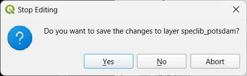
 uses an in-memory as data source.
 to open the Import Spectral Profiles window.

 and select the columns.
 symbol. The Export Spectral Library window will open.